9. Hypothesis Testing

Gordon E. Sarty

9. Hypothesis Testing

The process of hypothesis testing can be simplified into :

Transform (“reduce”) your given data into a test statistic that you can locate on probability distribution given by the sampling theory under a null hypothesis ( $H_{0}$ ) about the population. (e.g. $z,$ $t$ or $\chi^2$ test statistic).
See if your test statistic falls into a critical region of the distribution or not. The critical, or rejection region as we’ll call it, represents an area of low probability that the null hypothesis, $H_{0}$ is true. If the test statistic falls in the rejection region, the we make the decision to reject $H_{0}$ as the conclusion of the hypothesis test.

Before we define the critical region under the null hypothesis, we need to define what a null hypothesis is. We’ll define two hypotheses, actually, because the null hypothesis needs to contrasted to its logical opposite :

$H_{0}$ : Null Hypothesis, the hypothesis that nothing is going on; no effect; no signal.

$H_{1}$ : Alternative Hypothesis, the hypothesis that $H_{0}$ is not true; there is an effect; there is a signal.

A good experimental design will be set up so that the effects of interest define $H_{1}$ . (Your “claim” will be $H_{1}$ .) Why? It’s about signal to noise ratios. A test statistic is literally signal/noise, a signal to noise ratio. When you do not reject $H_{0}$ you are saying that there is more noise than signal. When you reject $H_{0}$ (essentially accepting $H_{1}$ ) you are saying that there is more signal than noise. Usually you are interested in the signal (also known as an “effect”) so your claim would be $H_{1}$ . You perform your experiment to find evidence for $H_{1}$ . If you are interested in noise (can happen, for example to test assumptions on which tests are based) then your claim would be $H_{0}$ . The examples that follow here don’t follow these experimentally correct rules for which of $H_{0}$ or $H_{1}$ should be the claim to emphasize the logical nature of the decision making process. But test statistics are signal to noise ratios and in real life you will be interested in signals.

To fix ideas about hypothesis testing, we’ll first look at hypotheses on the means of populations ( $\mu$ ). Later we’ll consider hypotheses on $\sigma$ and on $p$ (proportions).

With means there are three combinations of $H_{0}$ and $H_{1}$ to consider :

Two-Tailed Test

Right-Tailed Test

Left-Tailed Test

$H_{0}$ : $\mu = k$

$H_{0}$ : $\mu \leq k$

$H_{0}$ : $\mu \geq k$

$H_{1}$ : $\mu \neq k$

$H_{1}$ : $\mu > k$

$H_{1}$ : $\mu < k$

Here $k$ is a given number. Not that the rightness or the leftness of the one-tailed test is reflected in $H_{1}$ . $H_{1}$ is generally what people are interested in. Then the critical regions, which are on $z$ distributions as we’ll see, for each case look like :

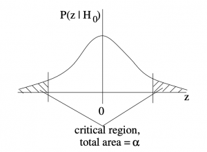
1. Two-tailed test:

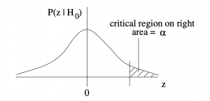
2. Right-tailed test:

3. Left-tailed test:

The critical regions, or rejection regions, appear in the probability distributions $P(z \mid H_{0})$ , which is the probability distribution that the sample test statistic, $z$ , that would occur if $H_{0}$ were true. These $z$ -distributions are $z$ -transforms of the distribution of sample means under $H_{0}$ given by the central limit theorem. More about this when we introduce the formula for the $z$ distribution. For now, let’s focus on the decision making process.

When your statistic ends up in the critical region, you conclude that $H_{0}$ is false. You reject $H_{0}$ . The critical region is the rejection region.

In the two tailed test, the critical region, with total area $\alpha$ is the opposite to the region ${\cal{C}} = 1 - \alpha$ that we have been using for confidence intervals. Compare the two-tail critical region sketch above to Figure 8.1.

There are four possible outcomes to a statistical hypothesis test given by the so-called^[1] “confusion matrix” :

$H_0$ true

$H_1$ true

Reject $H_{0}$ (believe $H_{1}$ )

Type I error $\alpha$

Correct decision 1- $\beta$

Do not reject $H_{0}$ (believe $H_{0}$ )

Correct decision 1- $\alpha$

Type II error $\beta$

The probabilities are relative to the realities. The probabilities in the columns add to 1. The probability of making a Type I error, $\alpha$ , is the area in the critical region. The diagram with the critical region on it assumes that $H_{0}$ is the reality. We will see how to compute $\beta$ in Chapter 13. The quantity $1- \beta$ is defined as the power of the statistical test.

We can view the confusion matrix from a medical test point of view. A medical test is a hypothesis test has the following hypotheses pairs :

$H_{0}$ : negative test result, healthy patient

$H_{1}$ : positive test result, sick patient

Then :

Healthy

Sick

Positive Result
(believe sick)

Type I error $\alpha$

Correct decision 1- $\beta$

Negative Result
(believe healthy)

Correct decision 1- $\alpha$

Type II error $\beta$

In medical tests, the quantity $1- \alpha$ is known as the test’s specificity, the probability of finding true negatives. The quantity $1 - \beta$ is the test’s sensitivity, the probability of finding true positives. Generally $\alpha$ and $\beta$ are functions of some other decision parameter. In the hypothesis tests that we consider here, $\alpha$ is the decision parameter.

Back to understanding the meaning of hypothesis testing. As we said, a good experimental design will be set up so that $H_{1}$ is your favourite theory that there is an effect. In that case $H_{0}$ represents the case that there is no effect : the position of $\bar{x}$ away from $k$ , or $z$ away from 0 (in the case of hypothesis testing of $\mu$ ) is just due to noise. If your experiment is then successful in proving your theory, i.e. you reject $H_{0}$ , then $\alpha$ represents the probability that you are wrong. The number $\alpha$ actually defines a decision point for rejecting $H_{0}$ . Later we will see how to compute a value, $p$ , that is associated with the test statistic. This $p$ -value is then a more refined value for the probability that you are wrong if you reject $H_{0}$ . From another point of view, $p$ would be the probability that your measurement is entirely due to noise.

Let’s do some examples to build our mechanical skills at defining critical regions for $z$ distributions.

Example 9.1 : Critical Areas on $z$ -distributions with hypothesis testing on the mean, $\mu$ .

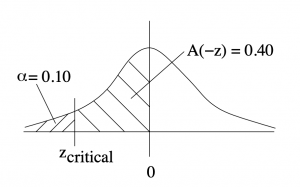
(a) Left-tailed test with $\alpha = 0.10$ . Find the critical value $z_{\rm critical}$ .

First step, draw a picture :

With the tables we have in the Appendix, there are two ways to find $z_{\rm critical}$ :

- Method (a) : Look up area in the Standard Normal Distribution Table equal to 0.40 : Closest $z$ is 1.28 so $z_{\rm critical} = -1.28$ .
- Method (b) : Use the last line in the t Distribution Table for the one tailed test column. Find a $z$ of 1.282 and add a minus sign because we have a left tail test. So $z_{\rm critical} = -1.282$ .

Use Method (b) on tests and exams. It is faster, requires less thinking about areas (and so less chance for making a mistake) and gives a slightly more accurate result. The critical area or critical region or the rejection region is where $z < -1.282$ . The critical value that defines the region in this case is $z = -1.282$ .

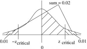
(b) A two tailed test with $\alpha = 0.02$ . Find the critical value $z_{\rm critical}$ .

Draw a picture :

- Method (a) : Look up area in the Standard Normal Distribution Table equal to 0.49. The closest $z$ is 2.33. So, because we have a two-tailed test, $z_{\rm critical} = \pm 2.33$ .
- Method (b): Use the last line in the t Distribution Table, for two tailed test, $\alpha = 0.02$ . Find $z = 2.326$ , $z_{\rm critical} = \pm 2.326$ .

Again, Method (b) is the recommended approach.

So the critical areas are those where

$z > 2.326 \mbox{ and } z < -2.326$

and the critical values are $z_{\rm critical} = 2.326$ and $z_{\rm critical} = -2.326$ .

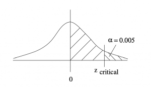
(c) A right tailed test with $\alpha = 0.005$ . Find the critical value $z_{\rm critical}$ .

Draw a picture :

- Method (a) Look up area in the Standard Normal Distribution Table equal to 0.495, the Closest $z$ is 2.58. So $z_{\rm critical} = 2.58$
- Method (b) Use the last line in the t Distribution Table for one tailed test, $\alpha = 0.005$ and find $z_{\rm critical} = 2.576$ .

So the critical area is that where $z > 2.576$ and the critical value is $z_{\rm critical} = 2.576$ .

▢

One final note on setting up the hypotheses. When setting up the hypotheses $H_{0}$ and $H_{1}$ , one of the two alternatives will be the claim (what the problem says you really want to test). As mentioned before, a good experimental design will have $H_{1}$ as the claim. But this may not always be possible to arrange (especially in tests of assumptions). So many of the exercises in the text and assignments will have $H_{0}$ as the claim.

So called not because it is confusing but because you are never 100 $\%$ sure which decision is correct. ↵

License

Icon for the Creative Commons Attribution-NonCommercial-ShareAlike 4.0 International License

Introduction to Applied Statistics for Psychology Students Copyright © 2022 by Gordon E. Sarty is licensed under a Creative Commons Attribution-NonCommercial-ShareAlike 4.0 International License, except where otherwise noted.

License

Share This Book