
7. The Central Limit Theorem
7.1 Using the Normal Distribution to Approximate the Binomial Distribution
Recall the definitions:  = probability of success,
  = probability of failure and
  = sample size. When
  and
and  then the normal distribution is very close, numerically, to the binomial distribution.
Using the histogram way of drawing the binomial distribution, a good fit looks like that shown in Figure 7.1.
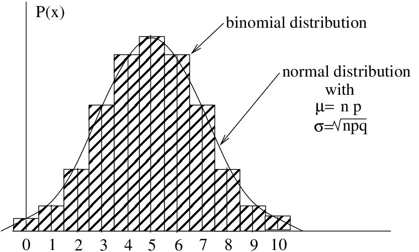
 and standard deviation
  is a good fit to the binomial distribution with the same mean and standard deviation as long as and .
A couple of things to note about this approximation:
- Although the values of the normal and the binomial distributions match well at
 equal to integer values when and , the areas match not as well. A “correction for continuity” can be used to better make the areas match but we won’t be worrying about such fine details in our studies.
 - We will use the normal approximation to the binomial make inferences on proportions. In that case , the probability of success will represent a proportion in a population.
