
14. Correlation and Regression
14.7 Confidence Interval for y′ at a Given x
At a fixed  (that is important to remember) the confidence interval for
  is
is
![\[ y^{\prime} - E < y < y^{\prime} + E \]](https://openpress.usask.ca/app/uploads/quicklatex/quicklatex.com-efb96205ae9d297cc2aeb3470a55b0f0_l3.png "Rendered by QuickLaTeX.com")
where
![\[ E = t_{\cal{C}} \; s_{\mbox{est}} \sqrt{1+ \frac{1}{n} + \frac{n(x - \overline{x})^{2}}{n(\sum x^{2})-(\sum x)^{2}}} \]](https://openpress.usask.ca/app/uploads/quicklatex/quicklatex.com-8eeb4fe78d300cc187a7dc10924b97f7_l3.png "Rendered by QuickLaTeX.com")
where, as usual,  comes from the t Distribution Table with
  .
.
Example 14.5 : Continuing from Example 14.4 (so you can see how an exam will go), say we want to predict the grade () in terms of a 95 confidence interval for the number of absences () equal to 10.
First, find the value predicted from the regression line, which we previously found to be :
![\[ y^{\prime} = 102.493 - 3.622 x \]](https://openpress.usask.ca/app/uploads/quicklatex/quicklatex.com-5b2aeac9eaf823b6621acc39663bee85_l3.png "Rendered by QuickLaTeX.com")
at  . The result is
![\[ y^{\prime} = 102.493 - 3.622 (10) = 66.273 \]](https://openpress.usask.ca/app/uploads/quicklatex/quicklatex.com-24ea1e2f489e378aca9471ecadafac43_l3.png "Rendered by QuickLaTeX.com")
Furthermore, from the last example, we found
![\[ s_{\mbox{est}} = 6.06 \]](https://openpress.usask.ca/app/uploads/quicklatex/quicklatex.com-eaf03ad012489ae9556cad1c6dcb6750_l3.png "Rendered by QuickLaTeX.com")
and, from the completed data table (Example 14.3)
![\[ \sum x = 57 \;\;\; \sum x^{2} = 579 \]](https://openpress.usask.ca/app/uploads/quicklatex/quicklatex.com-9e621d1db255d7f880598e8e5dd99cae_l3.png "Rendered by QuickLaTeX.com")
We still need  and
and  . Using our sums:
![\[ \overline{x} = \frac{\sum x}{n} = \frac{57}{7} = 8.143 \]](https://openpress.usask.ca/app/uploads/quicklatex/quicklatex.com-39743e20fa1f408cde8270688f43fb04_l3.png "Rendered by QuickLaTeX.com")
and from t Distribution Table for the 95 confidence interval,  we get
![\[ t{\cal{C}} = 2.571 \]](https://openpress.usask.ca/app/uploads/quicklatex/quicklatex.com-87347b4e63fdb9e7d00ee7546417f8d1_l3.png "Rendered by QuickLaTeX.com")
Now we compute  :
:

So

This is the 95 confidence interval for predicting the mark of a person who was absent for 10 days.
▢
Important:  is independent of but is not. So confidence intervals look like :
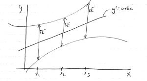
The reason for this variance of the width of the confidence interval comes from the uncertainty in the slope  . You can make plots like the one above in SPSS.
