
14. Correlation and Regression
14.2 Correlation
The correlation coefficient we will use here is called the “Pearson product moment correlation coefficient” and will be represented by the following symbols :
 — population correlation
 — sample correlation
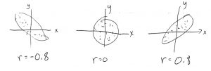
The correlation is always a number between  and
and  :
:  and
and  . If (or ) equals 0 then that means there is no correlation between
  and
and  . A minus sign means a minus slope, a plus sign means a positive slope.
The formula for is[1] :
(14.1) ![\begin{equation*} r = \frac{n(\sum xy) - (\sum x)(\sum y)}{\sqrt{[n (\sum x^{2}) - (\sum x)^{2}][n (\sum y^{2}) - (\sum y)^{2}]}} \end{equation*}](https://openpress.usask.ca/app/uploads/quicklatex/quicklatex.com-f42a06d446fb824fa57afa9ff42275d6_l3.png "Rendered by QuickLaTeX.com")
Example 14.1 : Compute the correlation between and for the data on Section 14.1 used for the scatter plot.
Solution : To compute , first make a table, fill in the data columns (on the right of the double vertical line below), fill in the other computed columns, sum the columns and finally plug the sums into the formula for :
| Subject | |
|
 |
 |
 |
|---|---|---|---|---|---|
| A | 6 | 82 | 492 | 36 | 6724 |
| B | 2 | 86 | 172 | 4 | 7396 |
| C | 15 | 43 | 645 | 225 | 1849 |
| D | 9 | 74 | 666 | 81 | 5476 |
| E | 12 | 58 | 696 | 144 | 3364 |
| F | 5 | 90 | 450 | 25 | 8100 |
| G | 8 | 78 | 624 | 64 | 6084 |
 |
 |
 |
 |
 |
 |
Plug in the numbers :
![\begin{eqnarray*} r & = & \frac{n(\sum xy) - (\sum x)(\sum y)}{\sqrt{[n (\sum x^{2}) - (\sum x)^{2}][n (\sum y^{2}) - (\sum y)^{2}]}}\\ & = & \frac{7(3745) - (57)(511)}{\sqrt{[7 (579) - (57)^{2}][7 (38993) - (511)^{2}]}}\\ & = & -0.944 \end{eqnarray*}](https://openpress.usask.ca/app/uploads/quicklatex/quicklatex.com-8c33bdfa75c01f4c580b61d150c875f8_l3.png "Rendered by QuickLaTeX.com")
Here there is a strong negative relationship between and . That is, as goes up, goes down with a fair degree of certainty. Note the is not the slope. All we know here, from the correlation coefficient, is that the slope is negative and the scatterplot ellipse is long and skinny.
▢
Standard warning about correlation and causation : If you find that and are highly correlated (i.e. is close to or ) then you cannot say that causes or that causes or that there is and causal relationship between and at all. In other words, it is true that if causes or that causes then will be correlated with but the reverse implication does not logically follow. So beware of looking for relations between variables by looking at correlation alone. Simply finding correlations by themselves doesn’t prove anything.
The significance of is assessed by a hypothesis test of
![\[ H_{0}: \rho = 0 \;\;\;\;\;\; H_{1}: \rho \neq 0 \]](https://openpress.usask.ca/app/uploads/quicklatex/quicklatex.com-edfdf158f522e99e4381e168093a89fd_l3.png "Rendered by QuickLaTeX.com")
To test this hypothesis, you need to convert to  via:
via:
![\[ t = r \sqrt{\frac{n-2}{1 - r^{2}}} \label{tcorrformula} \]](https://openpress.usask.ca/app/uploads/quicklatex/quicklatex.com-cf767c7cc96db4353406412ce607e865_l3.png "Rendered by QuickLaTeX.com")
and use  to find
  . The Pearson Correlation Coefficient Critical Values Table offers a shortcut and lists critical values that correspond to the critical values.
Example 14.2 : Given  ,
,  and
and  , test if is significant.
Solution :
1. Hypothesis. 
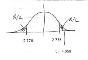
2. Critical statistic.
From the t Distribution Table with  and for a two-tailed test find
![\[ t_{\mbox{crit}} = \pm 2.776 \]](https://openpress.usask.ca/app/uploads/quicklatex/quicklatex.com-72919718908be95f9cd2f285a400ba2a_l3.png "Rendered by QuickLaTeX.com")
As a short cut, you can also look in the Pearson Correlation Coefficient Critical Values Table for ,  to find the corresponding
![\[ r_{\mbox{crit}} = \pm 0.811 \]](https://openpress.usask.ca/app/uploads/quicklatex/quicklatex.com-0bd2806c6065e466cfd5beb1287dd424_l3.png "Rendered by QuickLaTeX.com")
3. Test statistic.
![\[ t_{\mbox{test}} = r \sqrt{\frac{n-2}{1 - r^{2}}} = 0.897 \sqrt{\frac{6-2}{1 - (0.897)^{2}}} = 4.059 \]](https://openpress.usask.ca/app/uploads/quicklatex/quicklatex.com-e02446450370504b7c47e43d6cabdb78_l3.png "Rendered by QuickLaTeX.com")
4. Decision.
Using the :
or using the Pearson Correlation Coefficient Critical Values Table short cut :
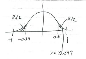
we conclude that we can reject  .
.
5. Interpretation. The correlation is statistically significant at .
▢
- The formula for is the same with all and in the population used. ↵
