15.3 SPSS Lesson 13: Proportions, Goodness of Fit, and Contingency Tables

Gordon E. Sarty

15. Chi Squared: Goodness of Fit and Contingency Tables

15.3 SPSS Lesson 13: Proportions, Goodness of Fit, and Contingency Tables

15.3.1 Binomial test

Up to now we haven’t seen how to use SPSS to handle tests of proportion. Recall that we used the $z$ approximation of the binomial distribution to do that test. SPSS can do the test using the binomial distribution directly. From the Data Sets, open “Cancer.sav” :

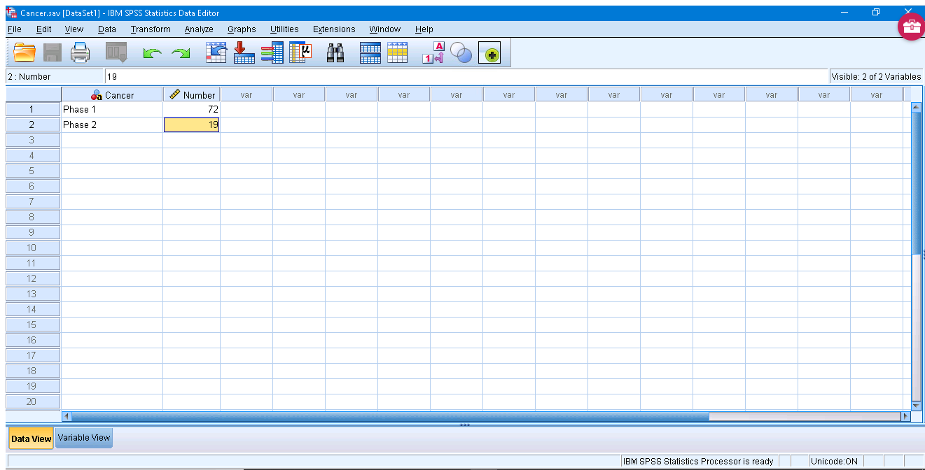
SPSS screenshot © International Business Machines Corporation.

Notice that the data are entered in frequency table form, so we need to tell SPSS this through the Data → Weight Cases menu and enter :

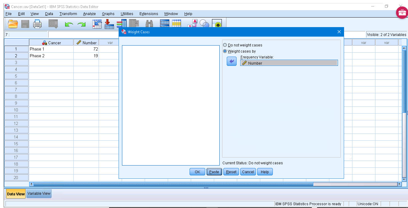
where the “Weight cases by” button has been pushed and the number variable has been identified as the frequency variable. Double check that “Weight On” appears at the lower right corner of the Data View pane. Now pick Analyze → Nonparametic Tests → Legacy Dialogues → Binomial to get and set :

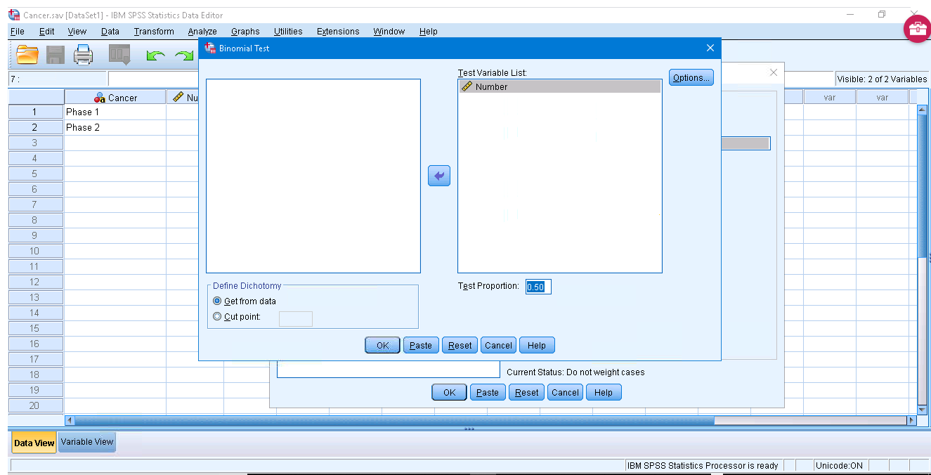
Alright, what are we doing here? We are doing a single sample proportions test where Other Door is the quality and proportion $p$ of interest and Door Behind is the quality proportion $q = 1-p$ not of interest. With Test Proportion set at 0.5, we are testing

$\begin{eqnarray*} H_{0} &:& p = 0.5 \\ H_{1} &:& p \neq 0.5 \end{eqnarray*}$

The output is straightforward:

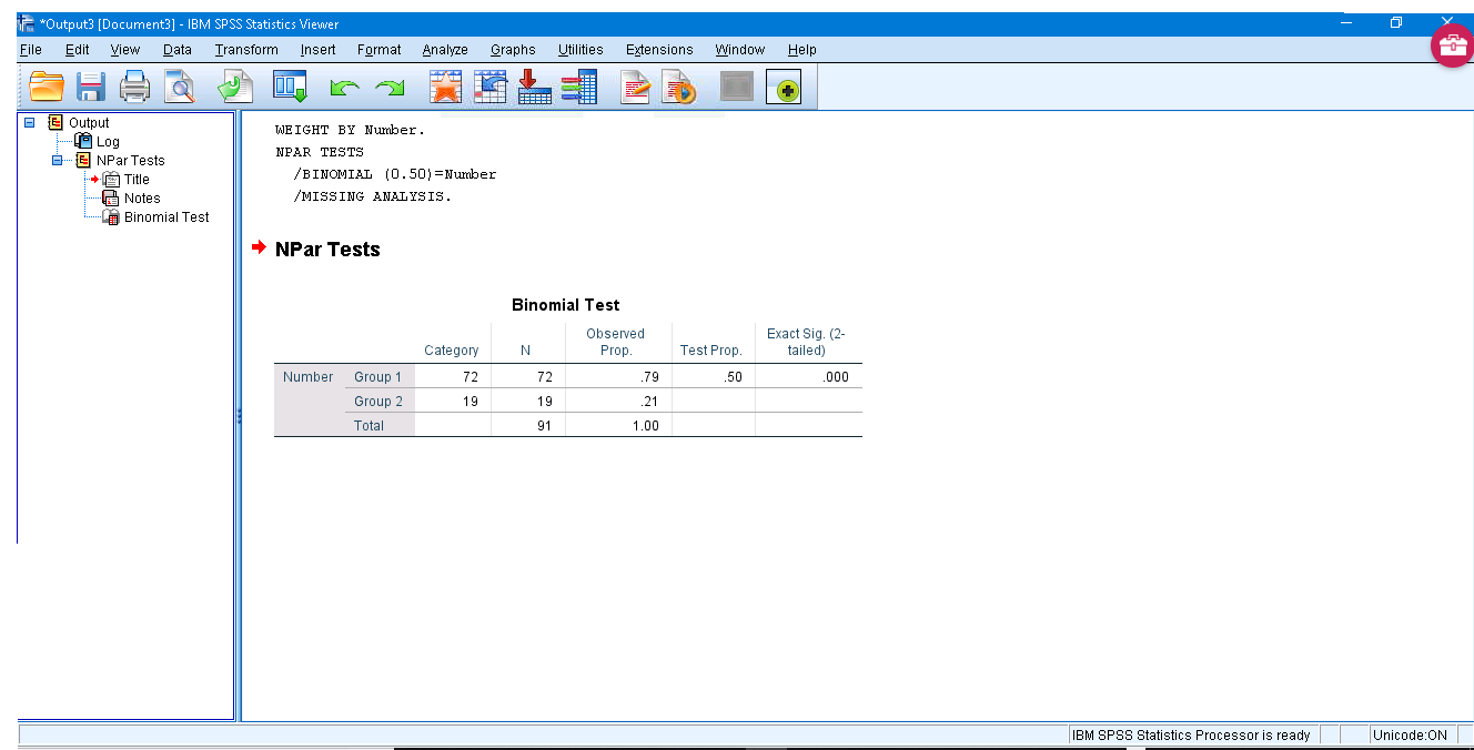
It says $\hat{p} = 0.79$ , $\hat{q} = 0.21$ and to reject $H_{0}$ .

15.3.2. $\chi^{2}$ goodness of fit test

From the Data Sets, open “CancerRecovery.sav” :

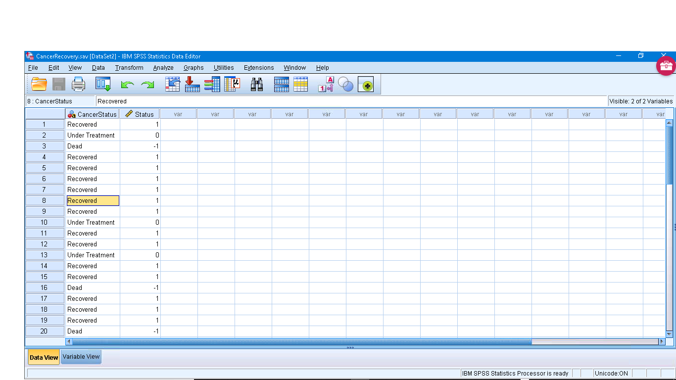
Going into the Variable View menu, you can check the number of qualitative values for each variable by looking at the Values attribute. For the Cancer status variable, the labels are :

-1 = “Dead”
0 = “Under Treatment”
1 = “Recovered”

Pick Analysis → Nonparametric Tests → Legacy Dialogues → Chi-square to get and set up :

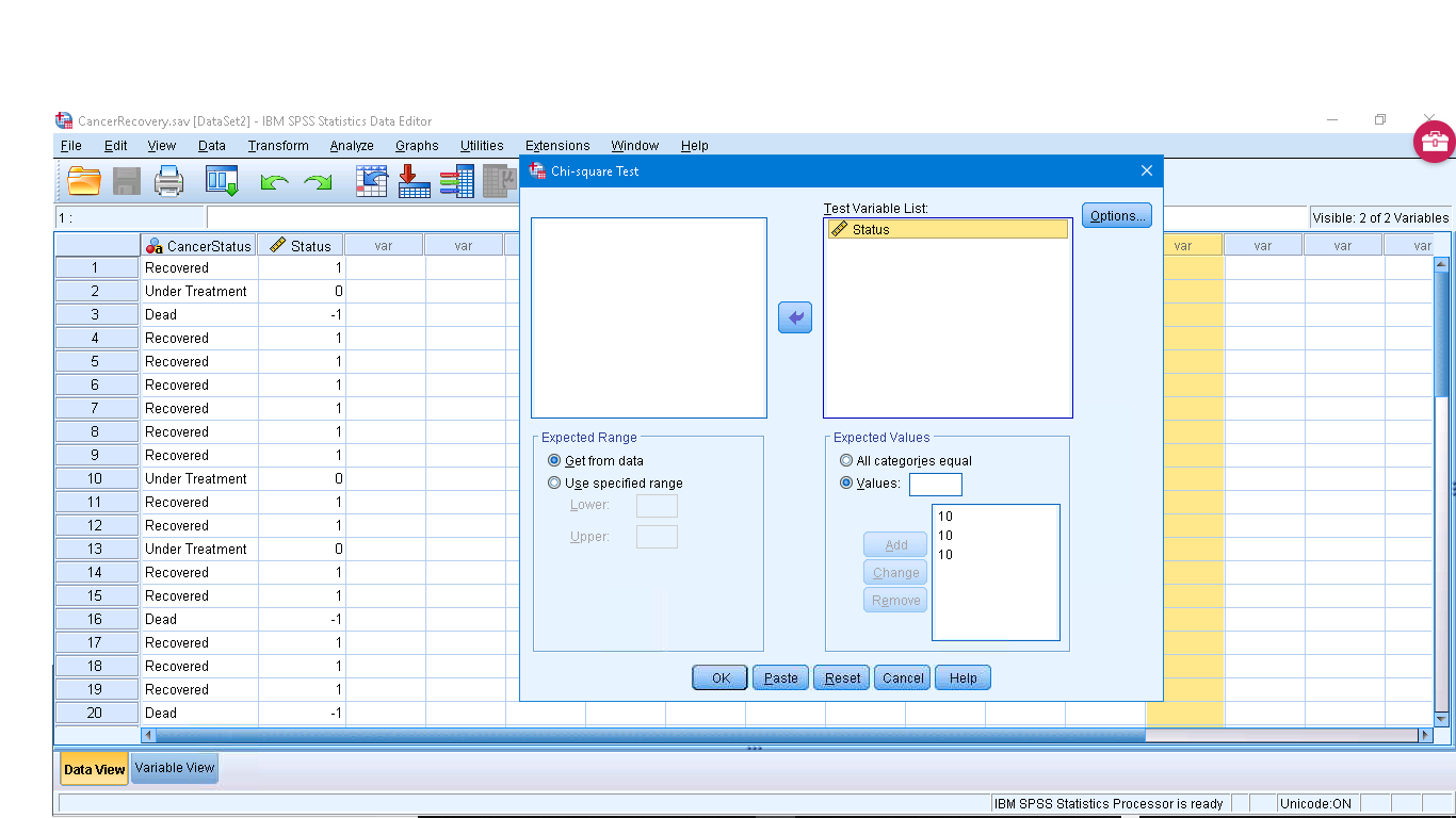
Here I have, somewhat randomly, explicitly set the expected frequencies. With the Expected Values button “All categories equal”, the expected frequencies will be $O_{i} = n/C = 30/3 = 10$ in this case. But I have set $O_{-1} = 10$ (for “less depressed”), $O_{0} = 10$ (for “same”), and $O_{1} = 10$ (for “more depressed”). (Make sure that $\sum O_{i} = n$ or who knows what SPSS will do.) The output is :

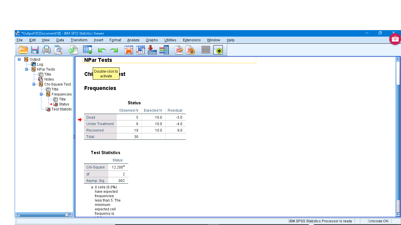
The first table lists the observed and expected frequencies explicitly. The second table gives $\chi^{2}_{\rm test} = 12.2$ , $\nu = C -1 = 2$ and $p = 0.002$ . So we (not unsurprisingly since I picked the expected frequencies randomly) reject $H_{0}:$ $E_{-1}=10, E_{0}=10, E_{1}=10$ .

15.3.3. Contingency tables: $\chi^{2}$ test of independence

From the Data Sets, open “CancerRecoveryAge.sav” :

Notice that the data are in frequency table form so I went into “weight cases” and chose number as the frequency variable — note the “Weight On” in the lower right corner. Explicitly the frequency table is the contingency table :

	Under 18	Between 18 and 50	Above 50
Dead	6	7	12
Under Treatment	7	7	9
Recovered	22	21	14

Notice that the sums of all the columns is 35 so this is a homogeneity of proportions set-up. Running the analysis is a little different. Pick Analysis → Descriptive Statistics → Crosstabs to get :

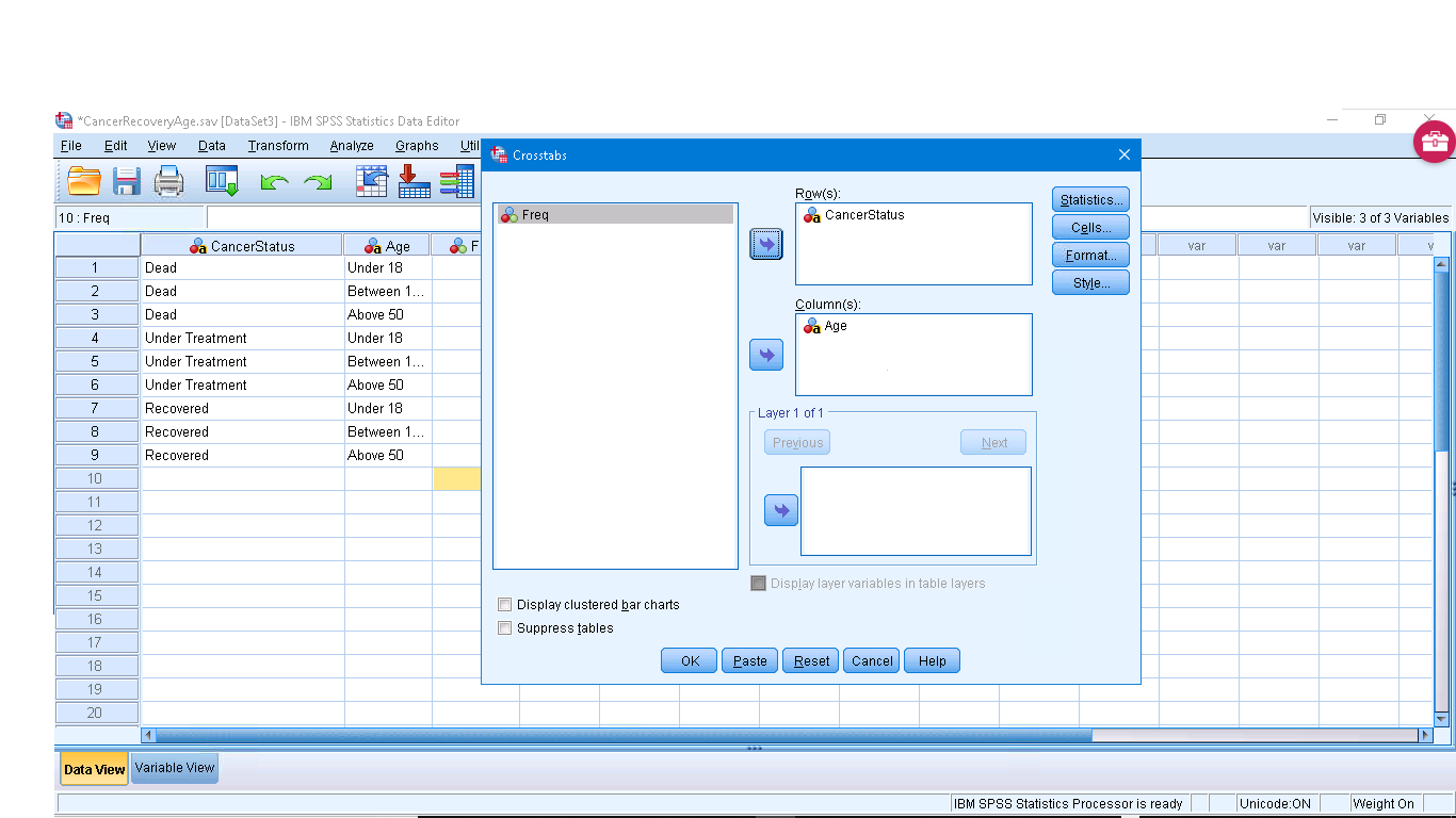
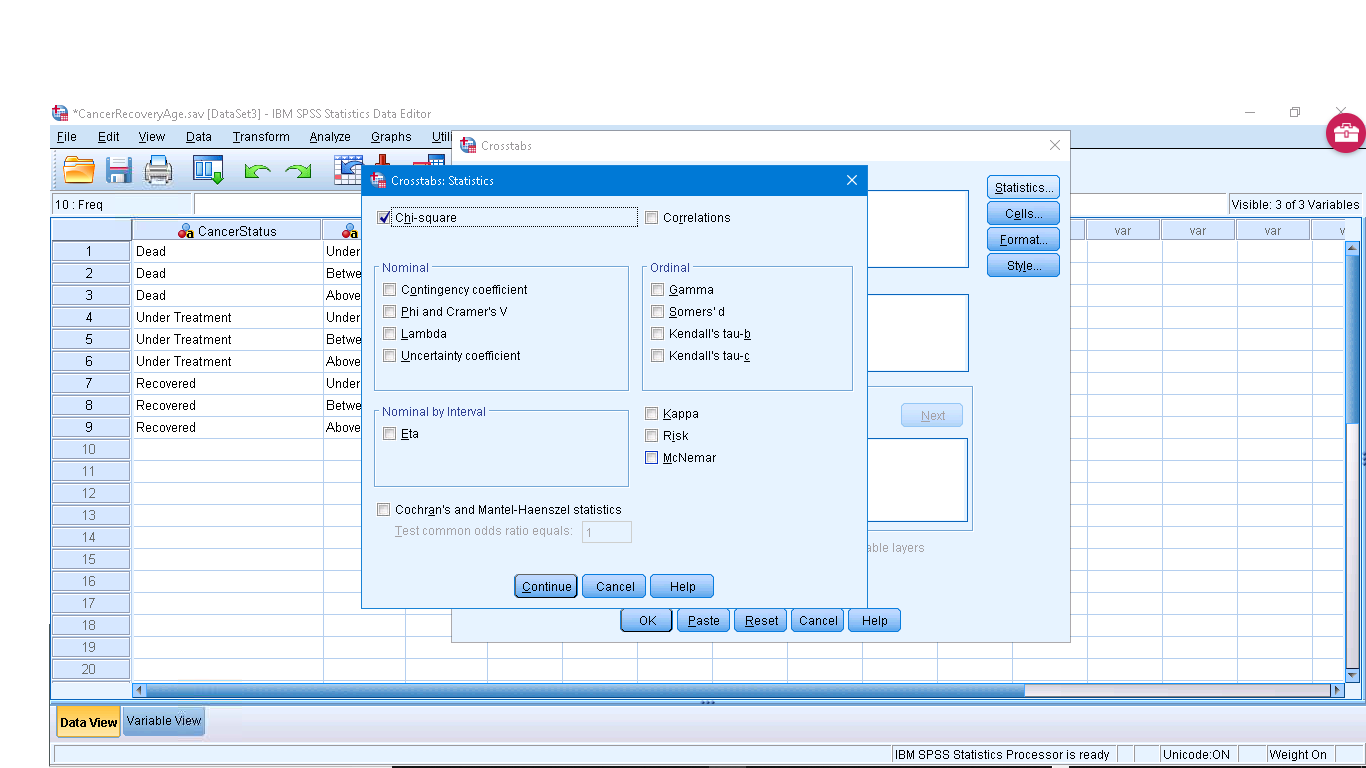
We need to set-up the submenus. First the Statistics menu, checkoff Chi-Square.

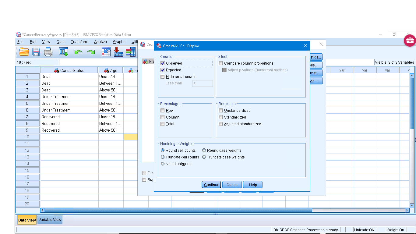
In Cells make sure Observed and Expected are checked :

Now you can run the analysis to get (ignoring the Case Processing Summary table) :

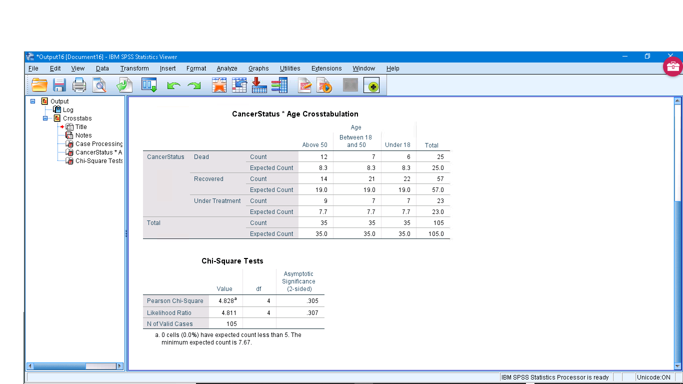
The first table is an explicit observed/expected frequency table with the row, column and total sums given. The second table gives $\chi^{2}_{\rm test} = 4.828$ , $\nu = (R-1)(C-1) = 4$ and $p = 0.305$ so we can not reject $H_{0}$ and conclude that “Deads” and “Under 18” are independent.