10.6 SPSS Lesson 6: Independent Sample t-Test

To follow along, load in the Data Set titled “pHLevel.sav”:

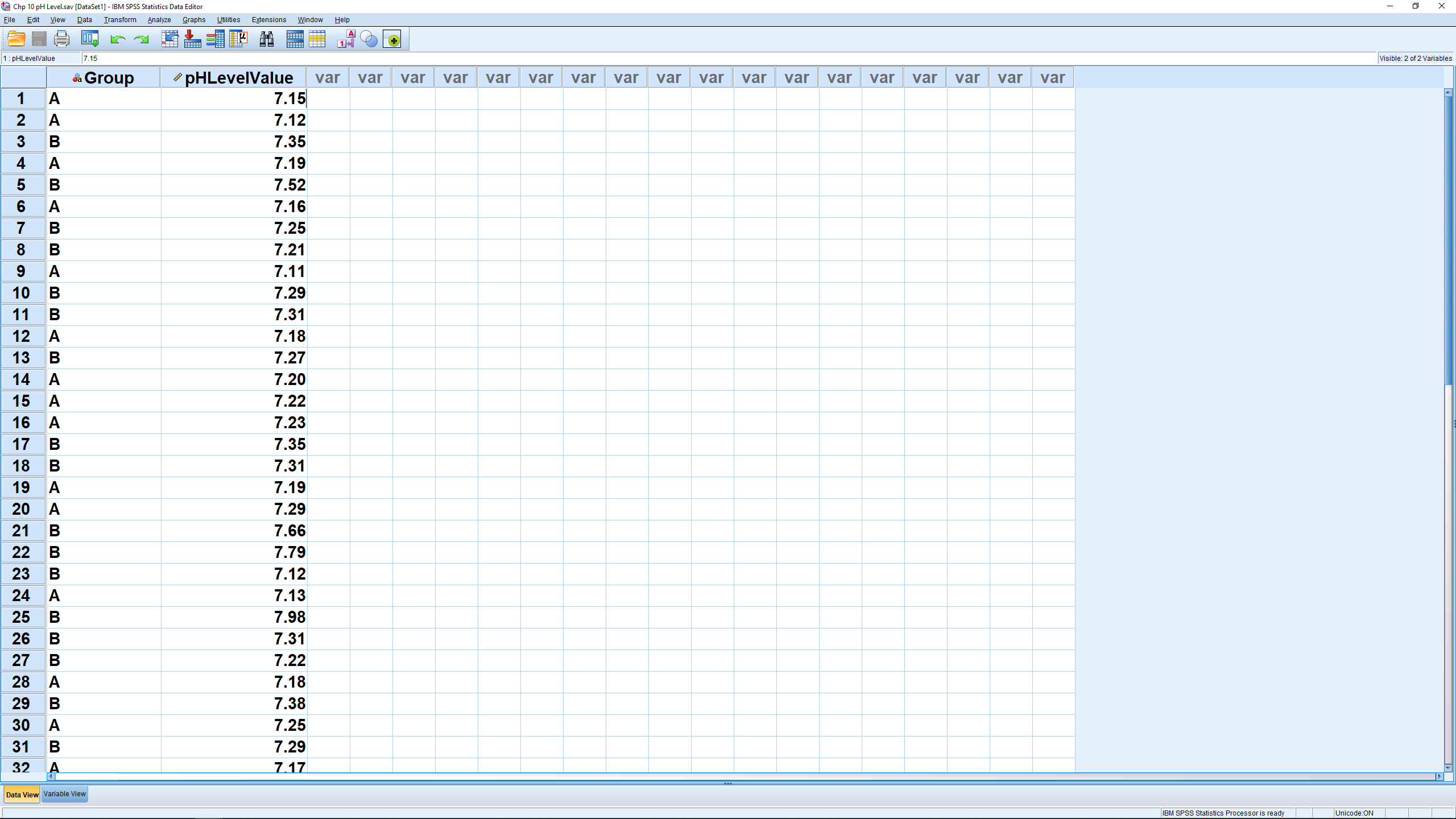
This is the first time we have an independent variable, Species in this case, and it has two values, setosa and versicolor, that label the two populations. Notice, especially, that we do not have separate columns for each sample. There is only one dependent variable, Sepal.Length in this case. As we cover the more advanced statistical tests in later chapters (part of PSY 234) the nature and complexity of the independent variable will evolve but we will always have just one independent variable.

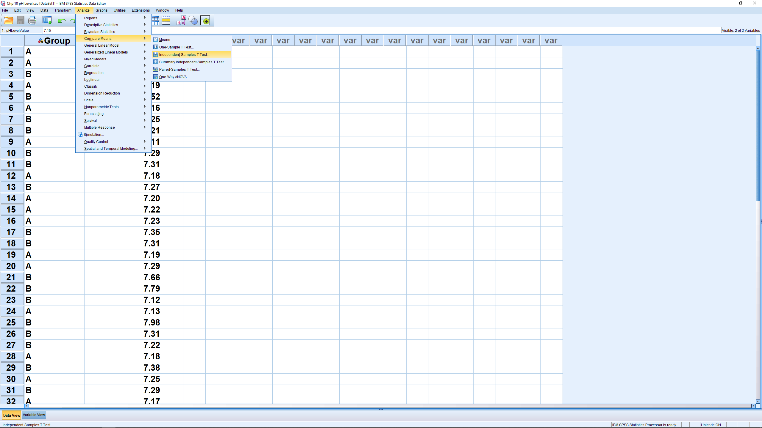
Running the -test is easy, pick Analyze Compare Means Independent Samples T Test :

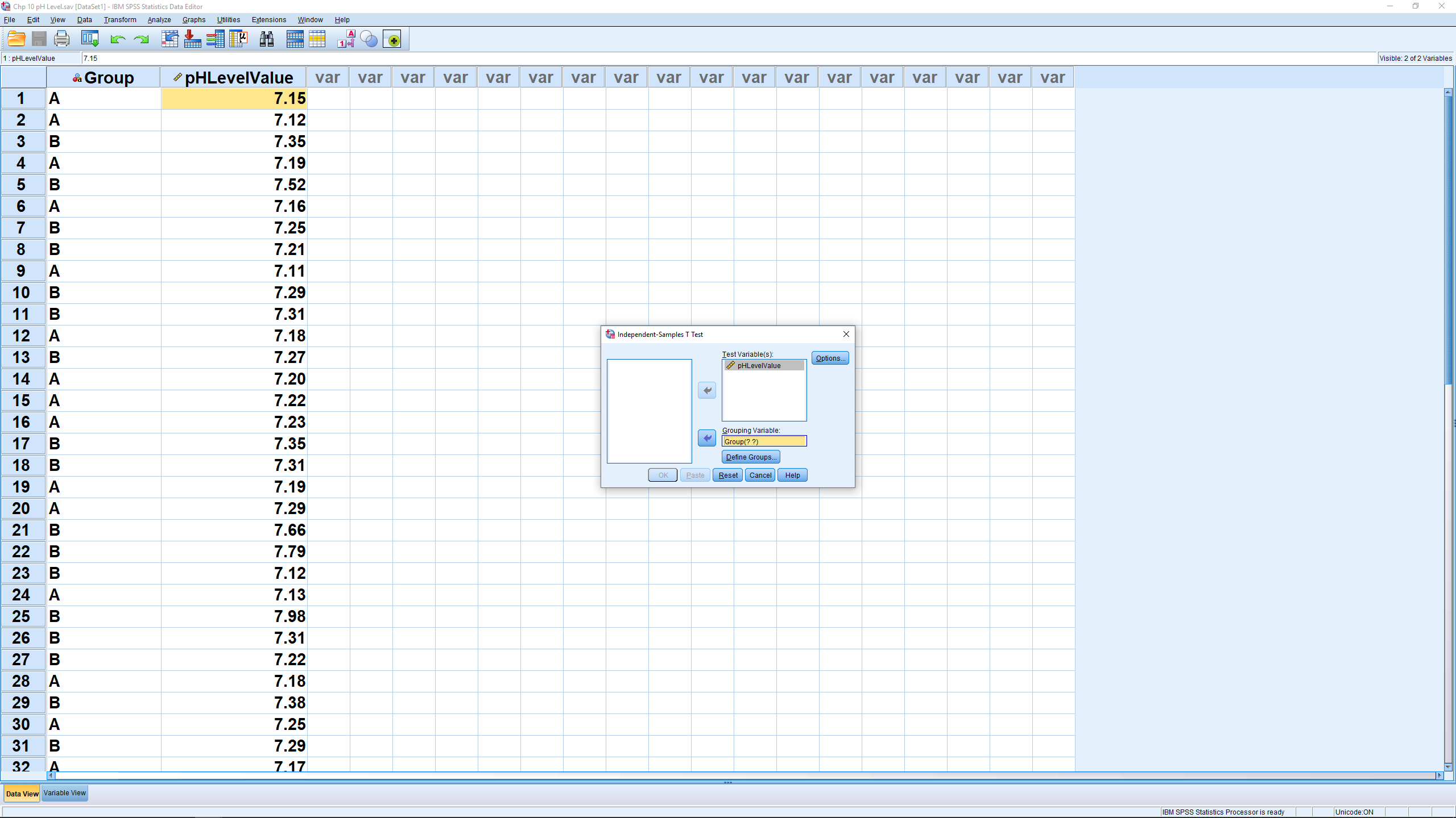
Select Sepal.Length as the Test Variable (dependent variable) and Species as the group variable (independent variable) :

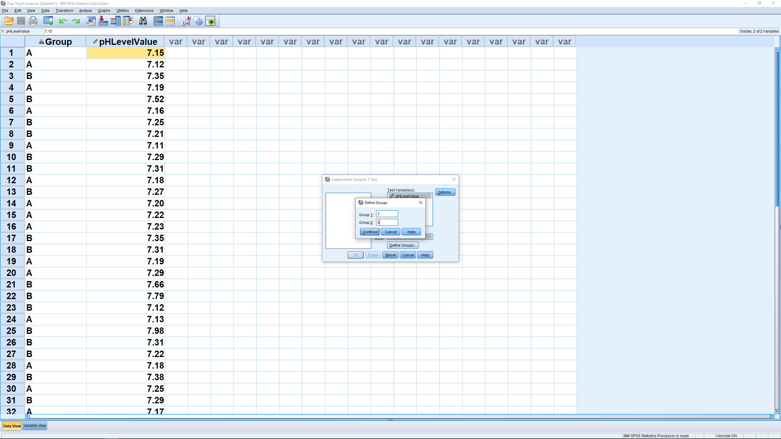
You need to do some work to let SPSS know that the two levels of the “grouping variable” are 1 and 2 (as can be seen in the Variable View window). So hit Define Groups… and enter:

Hit Continue, then OK (the Options menu will allow you to set the confidence level percent) to get:

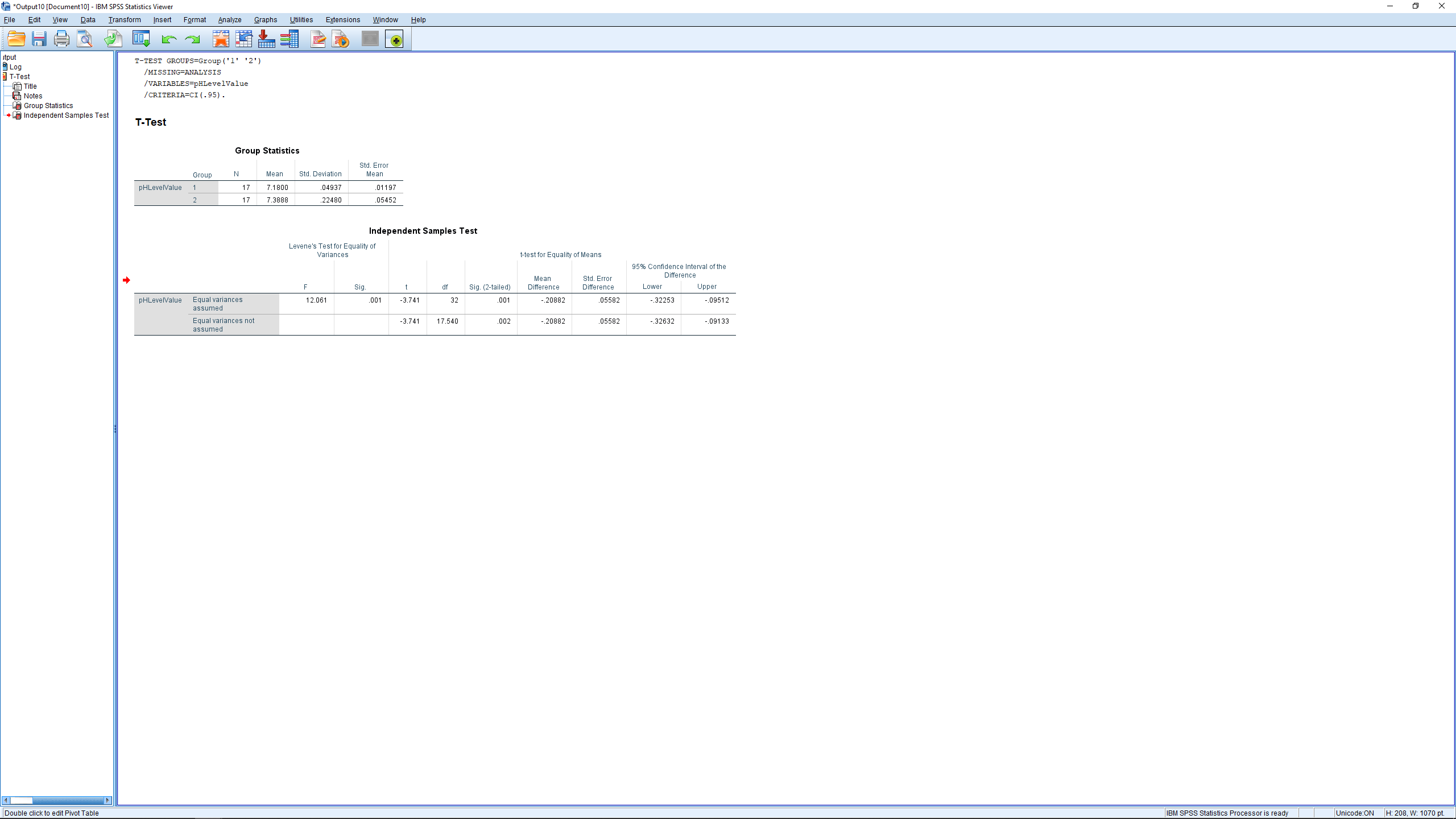
The first table shows descriptive statistics for the two groups independently. These numbers, excluding standard error numbers can be plugged into the formulae for pencil and paper calculations.

The important table is the second table. First, what hypothesis are we testing? It is important to write it out explicitly:

(10.6)  

This, as you recall, is our test of interest. When we did this test by hand, we had to do a preliminary test the see if we could assume homoscedasticity or not :

(10.7)  

That preliminary test is given to us as Levine’s test in the first two columns of the second table. Levine’s test is similar to but not exactly the same as the test we used but it also uses as a test statistic. Here we see with , so we reject and assume that population variances are unequal. That means we look at only the second line of the second table corresponding to “Equal variances not assumed”. SPSS computes and using both formulae but it does not decide for you which one is correct. You need to decide that yourself on the basis of the Levine’s test.

Again the information is fairly redundant. Looking across the second row we have (note that it is the same as the in the first row – that’s because the sample is large, making a good approximation for both), (notice the fractional here for the heteroscedastic case — recall Equation (10.3)), (note that it is for a two-tailed hypothesis, if your hypothesis is one-tailed then divide by 2), , and the standard error, the denominator of the test statistic formula ( is mean over standard error). The value is small, so we reject , the difference of the sample means is significant. The last two columns give the 95% confidence interval as

(10.8)  

Notice that zero is not in the confidence interval, consistent with rejecting .

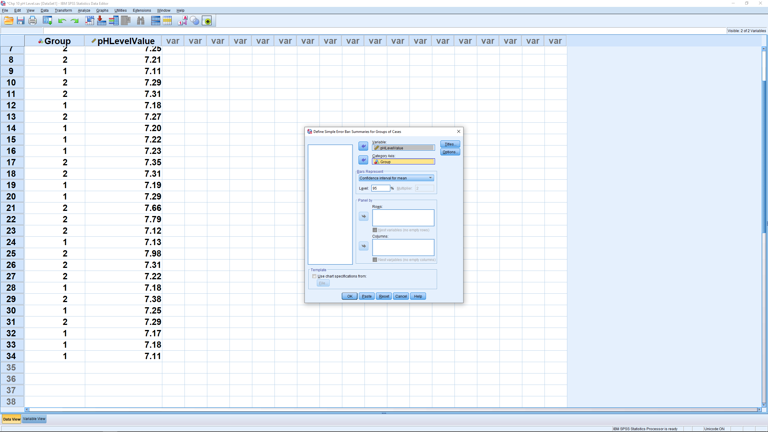
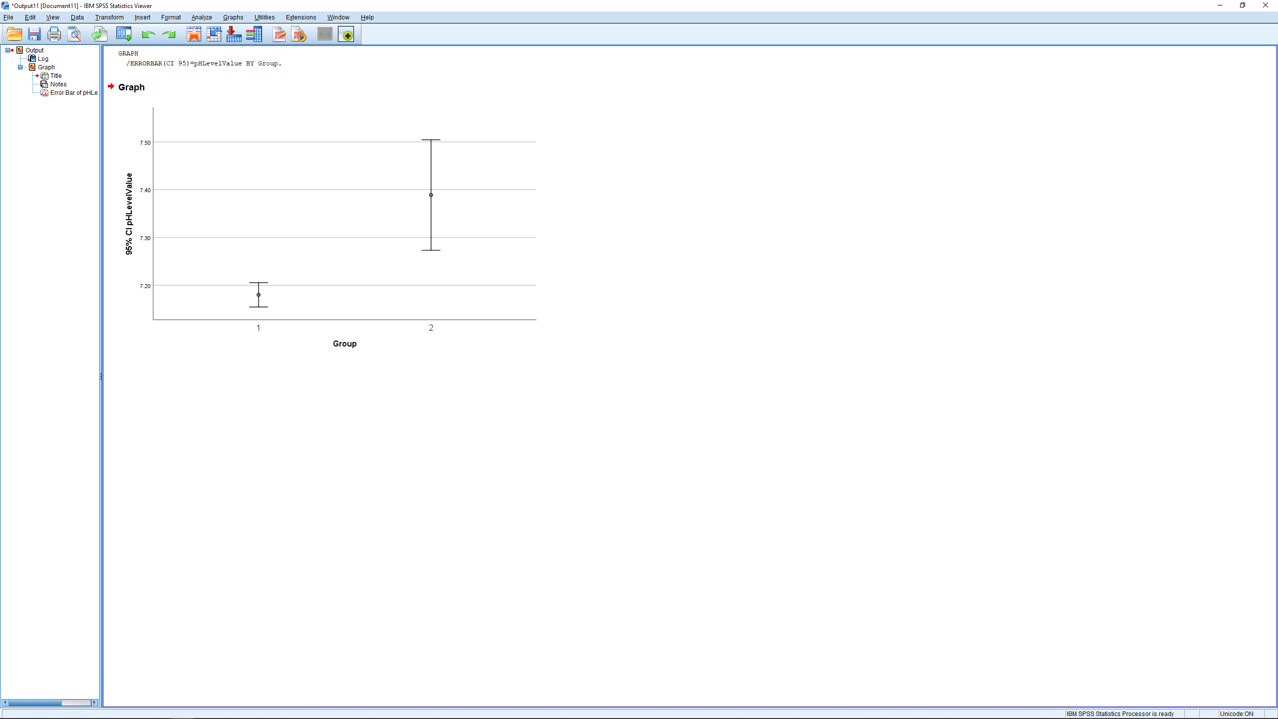
We can also make an error bar plot. Go through Graphs Legacy Dialogs Errorbar and pick Simple and “Summaries for groups of cases” in the next menu and:

which results in:

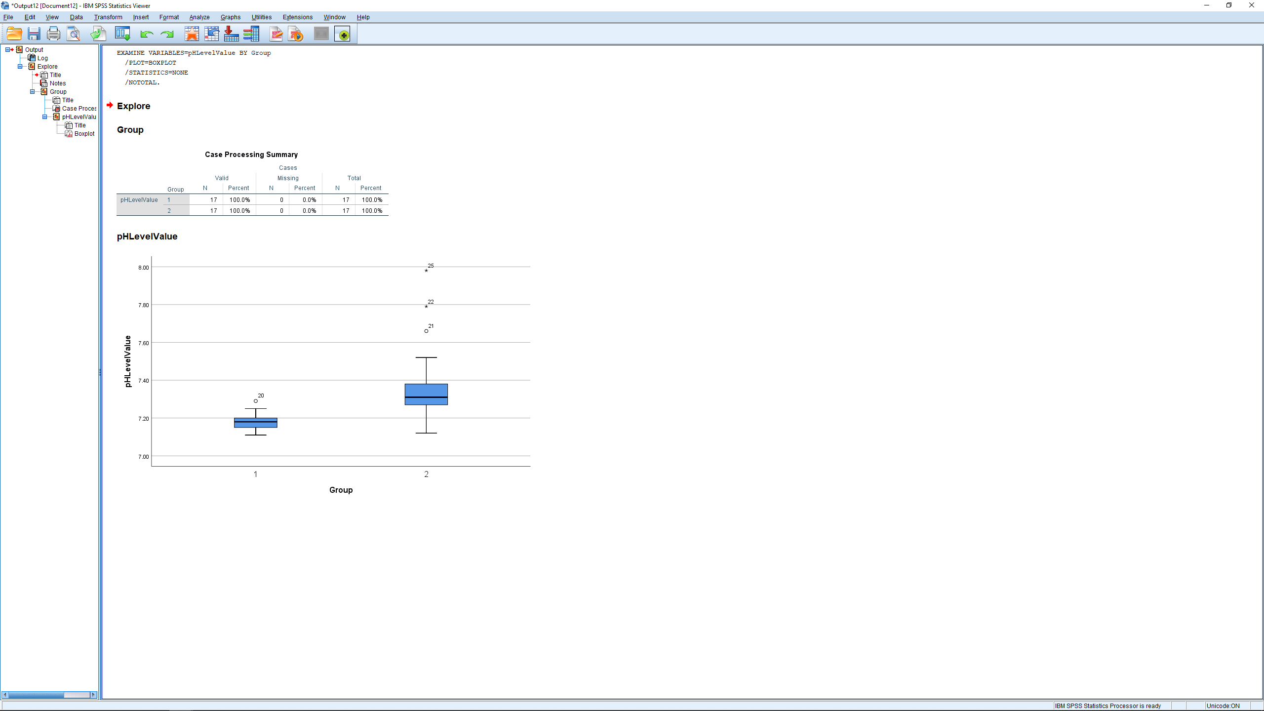
or you could generate a boxplot comparison:

Finally, we throw in a couple of effect size (descriptive) measures. One is the standardized effect size defined as:

(10.9)  

where is the pooled variance as given by Equation (10.4). Another measure is the strength of association

(10.10)  

which measures a kind of “correlation'” between and . The larger , the closer is to 1.