
15. Chi Squared: Goodness of Fit and Contingency Tables
15.2 Contingency Tables
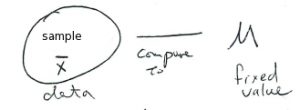
The goodness of fit test may be viewed as a frequency analogue of comparing a sample mean from one population to a hypothesized  mean,
mean,  , with the one-sample
  -test :
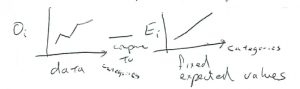
With the goodness of fit  test we compare an observed frequency profile with the (expected) frequency profile :
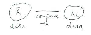
After studying the one-sample -test we moved on to the two-sample -test (and ANOVA) where we compared populations with each other directly :
Similarly, we will now move from comparing the observed frequencies from one group to a fixed profile to comparing the observed frequencies from several groups with each other :
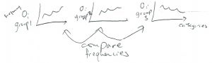
In the process we are testing to see if there is any relationship between the different groups and the categories labeled on the  axis.
axis.
To do this comparison, we need to make two contingency tables, one for the observed frequencies and one for the expected frequencies. The expected frequency table is computed from the values in the observed frequency table and not from some predetermined expected frequencies[1]. That way, the expected frequencies contingency table represents the frequencies expected if there were no difference between the groups.
The contingency table setup looks like :
.
| Group | |||||
| Category | 1 | 2 | 3 | 4 | |
| 1 | |||||
| 2 | |||||
| 3 | |||||
The numbers in the table will be frequencies. The contingency table has  rows with = number of categories and
  columns with = number of groups[2].
To compute the expected frequency table, we need to sum the rows and columns in the expected frequency table. We can write the sums at the ends of the rows and columns. So we will take our data and make the observed frequency contingency table :
| Group | ||||||
| Category | 1 | 2 | 3 | 4 | ||
| 1 |  |
 |
 |
 |
 |
|
| 2 |  |
 |
 |
 |
 |
|
| 3 |  |
 |
 |
 |
 |
|
 |
 |
 |
 |
 |
||
where  is the sum of row
  ,
,  is the sum of column
  and is the sum of all the entries in the table ( = sum of row sums = sum of column sums). Using the sums, the expected frequency table is :
| Group | |||||
| Category | 1 | 2 | 3 | 4 | |
| 1 |  |
 |
 |
 |
|
| 2 |  |
 |
 |
 |
|
| 3 |  |
 |
 |
 |
|
The expected frequency contingency table is the numerical expression of . In words: is the hypothesis that the groups and categories are independent. Therefore this contingency table test is called the test for independence.
The test statistic for this test is
![\[ \chi^{2} = \sum_{\mbox{all table entries }i,j} \frac{(O_{i,j} - E_{i,j})^{2}}{E_{i,j}} \]](https://openpress.usask.ca/app/uploads/quicklatex/quicklatex.com-a3aa0ff047ca276dad9aa86549f01fb7_l3.png "Rendered by QuickLaTeX.com")
with  where is the number of rows and is the number of columns.
Example 15.3 : Is there a relationship between the number of years spent in college and where you live? Test at  . The data, in table form are :
| years spent in college (group) | |||||
| No College | 4 yr degree | Advanced degree | sums | ||
| living location (category) | Urban | 15 | 12 | 8 | = 35 |
| Suburban | 8 | 15 | 9 | = 32 | |
| Rural | 6 | 8 | 7 | = 21 | |
| sums | = 29 | = 35 | = 24 | = 88 | |
In the table above, we have done some data reduction in summing the rows and columns. Continuing with the solution :
0. Data reduction. Compute the expected frequency table :
| No College | 4 yr degree | Advanced degree | |
| Urban |  |
 |
 |
| Suburban |  |
 |
 |
| Rural |  |
 |
 |
1. Hypotheses.
(Pay close attention to the wording.)
: Living location (category) is independent of the amount of education (group). : Living location (category) is dependent of the amount of education (group).
2. Critical statistic.
Use the Chi-Square Distribution Table with and
 to find
![\[ \chi^{2}_{\mbox{crit}} = 9.488 \]](https://openpress.usask.ca/app/uploads/quicklatex/quicklatex.com-8f2e7f09d947ad3592b12ff0768f5057_l3.png "Rendered by QuickLaTeX.com")
3. Test statistic.

4. Decision.
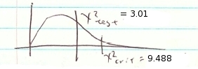
Do not reject .
5. Interpretation. The living location is independent of education.
▢
15.2.1 Homogeneity of proportions test
This test is a special case of the test of independence where the number of rows is always 2 and the total number of data points per column (the sum of frequencies per column) is the same for every column. With these restrictions we have a test that compares proportions between the populations represented by the columns. In particular, the test of independence generalizes the two-sample proportions test that we covered in Chapter 11. The first row of the contingency table represents  , the sample proportion of interest and the second row represents
  , the sample proportion not of interest. In using the homogeneity of proportions test, it is not necessary to explicitly compute the proportions .
Example 15.4 : We wish to test the hypothesis, at that different proportions of students in different high schools drive their own car given the following data :
| School 1 | School 2 | School 3 | sums | |
| Own Car | 18 | 22 | 16 | = 56 |
| Parent’s Car | 32 | 28 | 34 | = 94 |
| sums | = 50 | = 50 | = 50 | = 150 |
0. Data reduction. The first step in data reduction has been completed by summing the rows and columns. Using these sums, the expected frequencies are :
| School 1 | School 2 | School 3 | |
| Own Car | 18.67 | 18.67 | 18.67 |
| Parent’s Car | 31.33 | 31.33 | 31.33 |
1. Hypotheses :

2. Critical statistic.
Using the Chi-Square Distribution Table with and  find
find
![\[ \chi^{2}_{\mbox{crit}} = 5.991 \]](https://openpress.usask.ca/app/uploads/quicklatex/quicklatex.com-4e21fc04013ec7370beb15f1779595f8_l3.png "Rendered by QuickLaTeX.com")
3. Test statistic.
![\[ \chi^{2}_{\mbox{test}} = \sum_{table} \frac{(O - E)^{2}}{E} = 1.596 \]](https://openpress.usask.ca/app/uploads/quicklatex/quicklatex.com-8f4a62bc7fa7557da6c16511a9f8c8ec_l3.png "Rendered by QuickLaTeX.com")
4. Decision.
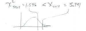
Do not reject .
5. Interpretation. We were unable to find any difference in the proportion of students who drive their own car between the schools at .
▢
 . This is the chance or completely random distribution for the expected frequencies.