17.1 Linear Algebra Basics

Gordon E. Sarty

17. Overview of the General Linear Model

17.1 Linear Algebra Basics

At its most abstract level modern mathematics is based on set theory. Functions, $f$ , are maps that map an element in a domain set, $D$ , to a target, $T$ .

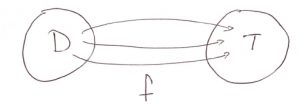
The range of of $f$ is the set $f(D)$ , the set of all possible values of $f$ . Note that the range is a subset of the target, in set notation symbols: $f(D) \subseteq T$ where $\subseteq$ means subset.

17.1.1 Vector Spaces

We specialize immediately to special sets called vector spaces and denote these sets by $\mathbb{R}^{n}$ . Here $n$ is the dimension of the vector space. Some examples :

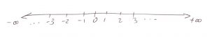
$\mathbb{R}^{1} = \mathbb{R}$ = the set of real numbers = the number line :

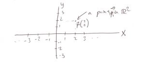
$\mathbb{R}^{2}$ = the set of all pairs of real numbers written as a column vector.

$\mathbb{R}^{2} = \left\{ \left. \left( \begin{array}{c} x \\ y \end{array} \right) \; \right| \; x,y \in \mathbb{R} \right\}$

We have introduced some set symbol notation here. The basic notion for a set uses curly brackets with a dividing line:

$\left\{ \mbox{symbols defining the set elements} \mid \mbox{details about the defining set symbols} \right\}$

The dividing line | is read as “such that”, and the set symbol $\in$ is read as “belongs to”, so you would read the set defining $\mathbb{R}^{2}$ above as: “the set of column vectors such that $x$ and $y$ belong to the set $\mathbb{R}$ “.

The transpose of a column vector is an operation written as

$\left( \begin{array}{c} x \\ y \end{array} \right)^{T} = \left( x \;\; y \right)$

…which is known as a row vector. The transpose of a row vector is a column vector.

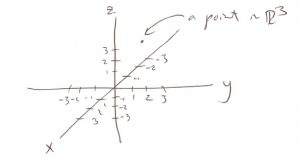
Continuing with higher dimensions:

$\mathbb{R}^{3} = \left\{ \left. \left( \begin{array}{c} x \\ y \\ z \end{array} \right) \; \right| \; x,y,z \in \mathbb{R} \right\} = \mbox{3D space}$

In general we have $n$ dimensional space^[1]:

$\mathbb{R}^{n} = \left\{ \vec{p} = \left. \left( \begin{array}{c} x_{1} \\ x_{2} \\ \vdots \\ x_{n} \end{array} \right) \; \right| \; x_{i} \in \mathbb{R}, \;\; i = 1, 2, \ldots, n \right\}$

Notice that we are using the symbol $\vec{p}$ to abstractly represent a column vector.

17.1.2 Linear Transformations or Linear Maps

In general we can define maps, $\ell$ , from $\mathbb{R}^{n} \rightarrow \mathbb{R}^{m}$ :

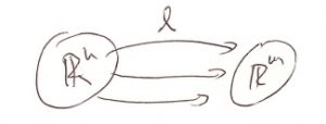
We will use the following abstract notation for a map: $\vec{q} = \ell(\vec{p})$ where $\vec{q} \in \mathbb{R}^{m}$ , $\vec{p} \in \mathbb{R}^{n}$ — $\vec{p}$ gets mapped to $\vec{q}$ by $\ell$ in this example.

A linear map or a linear transformation is a map that abstractly satisfies :

$a \ell(\vec{p}) + b \ell(\vec{q}) = \ell(a \vec{p} + b \vec{q})$

…where $a,b \in \mathbb{R}$ and $\vec{p}, \vec{q} \in \mathbb{R}^{n}$ (the domain of $\ell$ ). What this statement says is that, for a linear map, it does not matter if you do scalar multiplication and/or vector addition before (in $\mathbb{R}^{n}$ ) or after (in $\mathbb{R}^{m}$ ) the map $\ell$ , the answer will be the same. Scalar multiplication and vector addition^[2] are defined as follows, using example $\vec{p}, \vec{q} \in \mathbb{R}^{3}$ :

$\text{Scalar multiplication: } a \left( \begin{array}{c} x \\ y \\ z \end{array} \right) = \left( \begin{array}{c} ax \\ ay \\ az \end{array} \right)$

$\text{Vector addition: } \left( \begin{array}{c} x_{1} \\ y_{1} \\ z_{1} \end{array} \right) + \left( \begin{array}{c} x_{2} \\ y_{2} \\ z_{2} \end{array} \right) = \left( \begin{array}{c} x_{1}+x_{2} \\ y_{1}+y_{2} \\ z_{1}+z_{2} \end{array} \right)$

It turns out that any linear map from $\mathbb{R}^{n}$ to $\mathbb{R}^{m}$ can be represented by an $m \times n$ (rows $\times$ columns) matrix. Let’s look at some examples.

Example 17.1 : A map from $\mathbb{R}^{2}$ to $\mathbb{R}$ .

$z = \left[ \begin{array}{cc} 1 & 2 \end{array} \right] \left[ \begin{array}{c} x \\ y \end{array} \right] = (1)(x) + (2)(y)$

Here $\left[ \begin{array}{cc} 1 & 2 \end{array} \right]$ is a 1 $\times$ 2 matrix that defines a linear map $\ell : \mathbb{R}^{2} \rightarrow \mathbb{R}$ . The map $\ell$ takes the column vector $\left[ \begin{array}{c} x \\ y \end{array} \right]$ to the number $x + 2y$ in $\mathbb{R}$ . For example, the vector $\left[ \begin{array}{c} 2 \\ 3 \end{array} \right]$ gets mapped to 8. Notice how the matrix is applied to the vector. The row of the matrix is is matched to the column of the vector, the numbers are multiplied and then the column added.

▢

Example 17.2 : A map from $\mathbb{R}^{2}$ to $\mathbb{R}^{2}$ .

$\left[ \begin{array}{c} a \\ b \end{array} \right] = \left[ \begin{array}{cc} 1 & 2 \\ 3 & 4 \end{array} \right] \left[ \begin{array}{c} x \\ y \end{array} \right] = \left[ \begin{array}{c} x + 2y \\ 3x +4y \end{array} \right]$

Note that $\left[ \begin{array}{c} a \\ b \end{array} \right] = \left[ \begin{array}{cc} 1 & 2 \\ 3 & 4 \end{array} \right] \left[ \begin{array}{c} x \\ y \end{array} \right]$ gives us a nice compact way of writing the two equations:

$\begin{eqnarray*} a & = & x + 2y \\ b & = & 3x + 4y \end{eqnarray*}$

Linear algebra’s major use is to solve such systems of linear equations. Let’s try some numbers in $\left[ \begin{array}{c} a \\ b \end{array} \right] = \left[ \begin{array}{cc} 1 & 2 \\ 3 & 4 \end{array} \right] \left[ \begin{array}{c} x \\ y \end{array} \right]$ . Say $\left[ \begin{array}{c} x \\ y \end{array} \right] = \left[ \begin{array}{c} 1 \\ 1 \end{array} \right]$ , then:

$\left[ \begin{array}{c} a \\ b \end{array} \right] = \left[ \begin{array}{cc} 1 & 2 \\ 3 & 4 \end{array} \right] \left[ \begin{array}{c} 1 \\ 1 \end{array} \right] = \left[ \begin{array}{c} (1)(1)+(2)(1) \\ (3)(1)+(4)(1) \end{array} \right] = \left[ \begin{array}{c} 1+2 \\ 3+4 \end{array} \right] = \left[ \begin{array}{c} 3 \\ 7 \end{array} \right]$

…so $\left[ \begin{array}{c} 1 \\ 1 \end{array} \right]$ gets mapped to $\left[ \begin{array}{c} 3 \\ 7 \end{array} \right]$ .

▢

Example 17.3 : A map from $\mathbb{R}^{3}$ to $\mathbb{R}^{2}$

$\left[ \begin{array}{c} a \\ b \end{array} \right] = \left[ \begin{array}{ccc} 3 & 5 & 9 \\ 2 & 1 & 4 \end{array} \right] \left[ \begin{array}{c} x \\ y \\ z \end{array} \right] = \left[ \begin{array}{c} 3x + 5y + 9z \\ 2x + y + 4z \end{array} \right]$

Notice that the size of the matrix is 2 $\times$ 3 to give a map from $\mathbb{R}^{3}$ to $\mathbb{R}^{2}$ . Again this is shorthand for

$\begin{eqnarray*} a & = & 3x + 5y + 9z \\ b & = & 2x + y + 4z \end{eqnarray*}$

Let’s look at some numbers. Say $\left[ \begin{array}{c} x \\ y \\ z \end{array} \right] = \left[ \begin{array}{c} 2 \\ 4 \\ 3 \end{array} \right]$ , then:

$\left[ \begin{array}{c} a \\ b \end{array} \right] = \left[ \begin{array}{ccc} 3 & 5 & 9 \\ 2 & 1 & 4 \end{array} \right] \left[ \begin{array}{c} 2 \\ 4 \\ 3 \end{array} \right] = \left[ \begin{array}{c} (3)(2) + (5)(4) + (9)(3)\\ (2)(2) + (1)(4) + (4)(3) \end{array} \right] = \left[ \begin{array}{c} 6 + 20 + 27\\ 4 + 4 + 12 \end{array} \right] = \left[ \begin{array}{c} 53 \\ 20 \end{array} \right]$

…so $\left[ \begin{array}{c} 2 \\ 4 \\ 3 \end{array} \right]$ gets mapped to $\left[ \begin{array}{c} 53 \\ 20 \end{array} \right]$ .

▢

Exercises

Compute:

$\left[ \begin{array}{c} a \\ b \end{array} \right] = \left[ \begin{array}{cc} 5 & 2 \\ 1 & 2 \end{array} \right] \left[ \begin{array}{c} 1 \\ 2 \end{array} \right]$

$\left[ \begin{array}{c} a \\ b \\ c \end{array} \right] = \left[ \begin{array}{ccc} 10 & 2 & 1 \\ 5 & 1 & 4 \\ 1 & 1 & 1 \end{array} \right] \left[ \begin{array}{c} 2 \\ 3 \\ 2 \end{array} \right]$

$a = \left[ \begin{array}{ccc} 5 & 7 & 9 \end{array} \right] \left[ \begin{array}{c} 2 \\ 3 \\ 2 \end{array} \right]$

17.1.3 Transpose of Matrices

Just like vectors, matrices have a transpose where row and columns are switched. For example

$\left[ \begin{array}{ccc} 1 & 2 & 3 \\ 4 & 5 & 6 \end{array} \right]^{T} = \left[ \begin{array}{cc} 1 & 4 \\ 2 & 5 \\ 3 & 6 \end{array} \right]$

$\left[ \begin{array}{cc} 1 & 2 \\ 1 & 5 \end{array} \right]^{T} = \left[ \begin{array}{cc} 1 & 1 \\ 2 & 5 \end{array} \right]$

Note how, for square matrices (where the number of rows is the same as the number of columns), that transpose results in flipping numbers across the diagonal of the matrix.

17.1.4 Matrix Multiplication

An $(n \times p)$ matrix can be multiplied with a $(p \times m)$ matrix to give an $(n \times m)$ matrix. For example, we can multiply a $(3 \times 2)$ matrix with a $(2 \times 3)$ matrix to give a $(3 \times 3)$ matrix:

$\left[ \begin{array}{cc} 2 & 1 \\ 1 & 2 \\ 3 & 1 \end{array} \right] \left[ \begin{array}{ccc} 1 & 2 & 1 \\ 1 & 2 & 1 \end{array} \right] = \left[ \begin{array}{ccc} 3 & 6 & 3 \\ 3 & 6 & 3 \\ 4 & 8 & 4 \end{array} \right]$

Notice how the sizes of the matrices match so that the number of columns in the first matrix ( $p$ ) matches the number of columns in the second matrix — the $p$ ‘s kind of cancel to give the resulting $(n \times m)$ answer.

Matrix multiplication represents a composition of linear maps. In the above example the situation is:

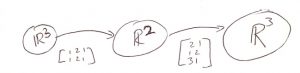
Note that the matrix on the right is applied first. (If you wanted to apply the matrices to a vector in $\mathbb{R}^{3}$ , you would would write the vector on the right.)

When you multiply two square matrices $[A]$ and $[B]$ (both $(n \times n)$ ) then, in general,

$[A] [B] \neq [B][A]$

Exercises

Compute:

$\left[ \begin{array}{ccc} 1 & 1 & 1 \\ 1 & 2 & 1 \\ 2 & 1 & 2 \end{array} \right] \left[ \begin{array}{ccc} 2 & 1 & 2 \\ 1 & 2 & 3 \\ 3 & 2 & 1 \end{array} \right]$

and

$\left[ \begin{array}{ccc} 2 & 1 & 2 \\ 1 & 2 & 3 \\ 3 & 2 & 1 \end{array} \right] \left[ \begin{array}{ccc} 1 & 1 & 1 \\ 1 & 2 & 1 \\ 2 & 1 & 2 \end{array} \right]$

to see that the results are different.

17.1.5 Linearly Independent Vectors

From an abstract point of view, a set of p vectors

$\vec{x}_{1}, \vec{x}_{2}, \ldots, \vec{x}_{p}$

in $\mathbb{R}^{n}$ are said to be linearly independent if the equation

$c_{1} \vec{x}_{1} + c_{2} \vec{x}_{2} + \cdots + c_{p} \vec{x}_{p} = 0$$

has only one solution:

$c_{1} = c_{2} = \cdots = c_{p} = 0$

When vectors are linearly independent, you cannot express one vector as a linear combination of the other vectors. Geometrically (for example in $\mathbb{R}^{3}$ ) :

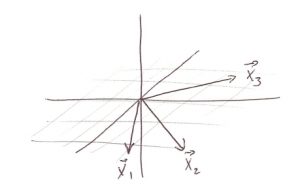
If $\vec{x}_{1}$ , $\vec{x}_{2}$ and $\vec{x}_{3}$ are all in the same plane then they are not linearly independent. In that case we could find $a$ and $b$ such that $\vec{x}_{3} = a \vec{x}_{1} + b \vec{x}_{2}$ .

In an $n$ dimensional space it is possible to take, at most, a set of $n$ linearly independent vectors.

17.1.6 Rank of a Matrix

Define :

Row rank = the number of linearly independent row vectors in a matrix.

Column rank = the number of linearly independent column vectors in a matrix.

It turns out that:

row rank = column rank = rank

We won’t cover the mechanics of how one calculates the rank of a matrix (take a linear algebra course if you want to know). Instead we just need to understand intuitively what the rank of a matrix means. Consider some simple examples :

Example 17.4 : The $(2\times 2)$ matrix

$\left[ \begin{array}{cc} 1 & 5 \\ 1 & 5 \end{array} \right]$

has rank = 1 because one column is a multiple of the other:

$5 \left[ \begin{array}{c} 1 \\ 1 \end{array} \right] = \left[ \begin{array}{c} 5 \\ 5 \end{array} \right]$

▢

Example 17.5 : The $(2 \times 2)$ matrix

$\left[ \begin{array}{cc} 1 & 1 \\ 1 & 2 \end{array} \right]$

has rank = 2 because there is no way to find $a$ such that

$\left[ \begin{array}{c} 1 \\ 2 \end{array} \right] = a \left[ \begin{array}{c} 1 \\ 1 \end{array} \right] = \left[ \begin{array}{c} a \\ a \end{array} \right]$

▢

Example 17.6 : The $(3 \times 3)$ matrix

$\left[ \begin{array}{ccc} 1 & 0 & 0 \\ 0 & 1 & 0 \\ 0 & 0 & 1 \end{array} \right]$

has rank = 3.

▢

Example 17.7 : The $(3 \times 3)$ matrix

$\left[ \begin{array}{ccc} 1 & 2 & 0 \\ 1 & 2 & 0 \\ 0 & 2 & 1 \end{array} \right]$

has rank = 2 since

$\left[ \begin{array}{c} 2 \\ 2 \\ 2 \end{array} \right] = 2 \left[ \begin{array}{c} 1 \\ 1 \\ 0 \end{array} \right] + 2 \left[ \begin{array}{c} 0 \\ 0 \\ 1 \end{array} \right]$

▢

17.1.7 The Inverse of a Matrix

For some square matrices ( $n \times n$ ) $[A]$ it is possible to find an inverse matrix, $[A]^{-1}$ so that

$[A][A]^{-1} = [A]^{-1} [A] = [I]$

where $[I]$ is the identity matrix that has 1 on the diagonal and 0 everywhere else.

For example, in $\mathbb{R}^{2}$ :

$[I] = \left[ \begin{array}{cc} 1 & 0 \\ 0 & 1 \end{array} \right]$

In $\mathbb{R}^{3}$ :

$[I] = \left[ \begin{array}{ccc} 1 & 0 & 0 \\ 0 & 1 & 0 \\ 0 & 0 & 1 \end{array} \right]$

In $\mathbb{R}^{4}$ :

$[I] = \left[ \begin{array}{cccc} 1 & 0 & 0 & 0 \\ 0 & 1 & 0 & 0 \\ 0 & 0 & 1 & 0 \\ 0 & 0 & 0 & 1 \end{array} \right]$

…etc.

Again, we won’t learn how to compute the inverse of a matrix but it is important to know that an $(n \times n)$ matrix $[A]$ will have an inverse $[A]^{-1}$ if and only if rank $([A]) = n$ .

17.1.8 Solving Systems of Equations

In general a system of linear equations can be represented by

$\vec{y} = [A] \vec{x}$

where $\vec{y} \in \mathbb{R}^{n}$ , $\vec{x} \in \mathbb{R}^{p}$ and $[A]$ is an $(n \times p)$ matrix known as the {\em coefficient matrix}. Here $\vec{y}$ represents the known values and $\vec{x}$ represents the unknown values.

There are 3 cases:

$n < p$ , less equations than unknown. No unique solution.
$n = p$ , number of equations = number of unknowns.

Rank $[A] < n$ , no unique solution. This is really the same as case 1 because at least one of the equations is redundant.
Rank $[A] = n$ . This has the unique solution $\vec{x} = [A]^{-1} \vec{y}$ .

3. $n > p$ , more equations than unknowns.

Rank $[A] < p$ , inconsistent formulation, no solution possible.
Rank $[A] = p$ ( $[A]$ is of full rank). A least squares solution is possible and is given by :

$\vec{x} = ([A]^{T} [A])^{-1} [A]^{T} \vec{y}$

That last least squares solution is the punchline to this very quick overview of linear algebra. It is derived using differential calculus in the same way that least squares solutions were derived for linear and multiple regression. The existence of this least squares solution allows us to unify many statistical tests into one big category called the General Linear Model.

The number $n$ will also mean sample size later on because you can organize a data set into a column vector of dimension $n$ . In fact, you give SPSS a data vector by entering a column of numbers as a "variable" in the input spreadsheet. ↵
Abstractly, a vector space is a set where scalar multiplication and vector addition can be sensibly defined. ↵

License

Icon for the Creative Commons Attribution-NonCommercial-ShareAlike 4.0 International License

Introduction to Applied Statistics for Psychology Students Copyright © 2022 by Gordon E. Sarty is licensed under a Creative Commons Attribution-NonCommercial-ShareAlike 4.0 International License, except where otherwise noted.

17.1.1 Vector Spaces

17.1.2 Linear Transformations or Linear Maps

Exercises

17.1.3 Transpose of Matrices

17.1.4 Matrix Multiplication

Exercises

17.1.5 Linearly Independent Vectors

17.1.6 Rank of a Matrix

17.1.7 The Inverse of a Matrix

17.1.8 Solving Systems of Equations

License

Share This Book