12.5 Two-way ANOVA

Gordon E. Sarty

12. ANOVA

12.5 Two-way ANOVA

In all the statistical testing we’ve done so far, and will do in Psy 233/234, there is only one dependent variable (DV) — we have been/are doing univariate statistics.

And so far, in all the tests we’ve seen there has only been one independent variable (IV). For the $t$ -tests the IV is group or population with only two values^[1] 1 and 2. In one-way ANOVA the single IV has $k$ (number of groups) values. Also, so far, the IV has been a discrete variable (that will change when we get to regression). The graph to keep in mind for the one-way ANOVA is a profile graph as shown in Figure 12.1.

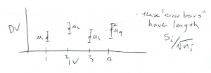
Figure 12.1: The profile plot is a good way to think of one-way ANOVA data with the IV on the $x$ -axis and the DV on the $y$ -axis. A one-way ANOVA tests the hypothesis: are all the means $\mu_{i}$ equal to each other? (An actual data profile graph can only have sample values $\overline{x}_{i}$ , we show a kind of confidence interval plot here.)

With two-way ANOVA you have two IVs. Let’s call the two IVs $A$ and $B$ . Each IV in two-way ANOVA is called a factor. $A$ and $B$ can each have several values (or “levels”). To introduce concepts, let’s stick with the case were each of $A$ and $B$ hove only 2 values: $A_{1}$ and $A_{2}$ for $A$ , and $B_{1}$ and $B_{2}$ for $B$ . This is the $2\times2$ ANOVA case, where the 2 tells you haw many levels are in each factor. If, for example, $A$ had 4 levels (values) and $B$ had 3 levels then you’d have a $4\times3$ ANOVA. Let’s stick with the $2\times2$ case for now.

There are several ways to think of a two-way ANOVA. Let’s start with two-dimensional profile plots for a $2\times2$ ANOVA :

The profile plot can be done in one of two ways. The $y$ axis represents the DV in both cases. On the left, the $x$ axis represents the IV $A$ and the two values of the other IV, $B$ , are represented as lines. On the right, the $x$ axis represents the IV $B$ and the two values of the other IV, $A$ , are represented as lines. Look closely at the plots. The dots represent the population values^[2] with $\mu_{i,j}$ being the value of the population labelled by $A=i,B=j$ . The means in the two plots are exactly the same. Each combination of IVs, $i,j$ , defines a treatment group. For a $2\times2$ ANOVA there are four treatment groups.

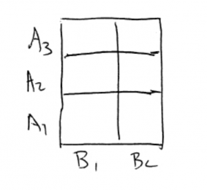
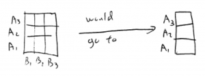
Two way ANOVA supposedly had one of its first applications to agriculture. So, to fix ideas, let’s take our two IV’s, also known as two factors as :

$\begin{eqnarray*} A & = & \mbox{ Plant food type} \nonumber \\ B & = & \mbox{ Soil type} \nonumber \end{eqnarray*}$

Then, with two levels for each factor, we can visualize the setup as fields where you would grow plants :

Each field, or treatment group, is also known as a cell.

Now, lets use the $x$ and $y$ axes to represent the IVs ( $B$ and $A$ in this case). Then we can use the $z$ axis to represent the DV in a 3D plot :

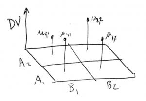
This makes sense. A two-way ANOVA has three variables, two IVs and on DV, so the data are 3D data and the plot above shows how those data appear in 3D space. If you look at the 3D plot from the front you see the profile plot with $B$ on the $x$ axis. If you look at the 3D plot from the (right) side, you see the profile plot with $A$ on the $x$ axis.

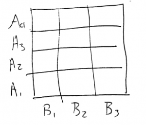
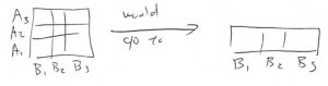
We’ve focused on $2\times2$ designs. But the two IVs can have any number of discrete values or levels. For example, a $3\times2$ cell diagram would look like :

And a $4\times3$ design would look like :

Now that we understand what kind of data we have, it’s time to move onto hypothesis testing. In two-way ANOVA there are three hypotheses to test :

Is there a “main effect” of $A$ ?
Is there a “main effect” of $B$ ?
Is there an interaction of $A\times B$ ?

In all cases, $H_{0}$ is that there is no effect or interaction. As we will see, each hypothesis is a one-way ANOVA of the two-way data suitably collapsed into a one-way design. Let’s begin with the main effect of $A$ . The hypothesis is equivalent to collapsing the design across $B$ :

and then doing a one-way ANOVA with the one IV equal to $A$ . The collapse is done by averaging over $B$ which is the same as removing the cell boundaries between the $B$ cells and only categorizing the data by the $A$ levels.

The hypothesis for the main effect of $B$ is similarly equivalent to collapsing across $A$ :

and then doing a one-way ANOVA with the one IV equal to $B$ .

The hypothesis test for the interaction is a one-way ANOVA on the “difference of differences”. The idea in interpreting a significant^[3] interaction is that the effect of changing IV $A$ depends on the effect of changing $B$ . Let’s see how the differences arise in a $2\times2$ ANOVA :

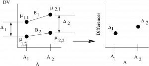
The interaction tests if there is a significant difference between the two differences $\Delta_{1} = (\mu_{1,1} - \mu_{1,2})$ and $\Delta_{2} = (\mu_{2,1} - \mu_{2,2})$ . Note that I could have set up the differences on the profile plot with $B$ on the $x$ axis. It does not matter, the resulting one-way ANOVA turns out to be the same. For $A \times 2$ or $2 \times B$ ANOVAs you get more than two differences to compare with a one-way ANOVA. With a generic $A \times B$ ANOVA you need to take a mean of differences to compare to each other. The interpretation of a generic $A \times B$ can be tricky.

The interpretation of $2\times2$ interactions is, however, pretty straightforward. You need to consider all the possible outcome of the $2\times2$ ANOVA with its three hypotheses. Since any hypothesis can be significant or not we have $2^{3} = 8$ possible outcomes^[4]. Let’s look at generic cases of all the combinations of the outcomes of a $2\times2$ ANOVA using $A$ , $B$ and $A \times B$ to denote that $H_{0}$ has been rejected and significant effects have been found :

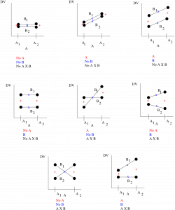
The first thing to remember about these diagrams is that they are for interpretation — for step 5 of our hypothesis testing procedure. You have to do the actual hypothesis test with three $F_{\mbox{test}}$ statistics to decide which case you have. Secondly, note that the graphs are generic. In statistics numbers are fuzzy. That is, every mean is fuzzy by a standard deviation. So think of the dots on the graphs as fuzzy balls and that the lines do not have to go to the centers of the fuzzy balls. Now look at the + and x symbols. The + symbols show what happens when you collapse the design over $B$ to see the main effect of $A$ ; what is left are the two averages^[5] for $A_{1}$ and $A_{2}$ . The two + means are then compared with a one-way ANOVA (essentially a $t$ -test since $t^{2}_{\nu} = F_{1, \nu}$ ) to see if there is a main effect of $A$ . Similarly the x symbols show what happens when you collapse the design across $A$ to see the main effect of $B$ . The means for $B_{1}$ and $B_{2}$ will be halfway^[6] along the $B_{1}$ and $B_{2}$ lines. The two x means are then compared with a one-way ANOVA to see if there is a main effect of $B$ . Finally lets look at the interactions. There are four cases in the diagrams that show interactions. In two cases the diagrams have crossed lines where the differences at either end are the negative of each other (and so are different) and in two cases the magnitudes of the differences are different. Looking at all the cases we see that there will be an interaction if the lines are not statistically parallel. The concept of statistically parallel is important here. Your actual data profile plot may not look like it has parallel lines but there will be no significant interaction if the lines are not statistically distinguishable from being parallel — this is the information that the hypothesis test gives you.

Before we move on, let’s consider post-hoc testing for two-way ANOVAs. This usually means comparing means pairwise cell by cell. As with one-way ANOVA that would mean also finding a suitable correction for the $p$ -value if $t$ -tests are used. We won’t cover post-hoc testing for two-way ANOVAs in any detail here except to point out that post hoc testing for a $2 \times 2$ ANOVA is redundant. A $2 \times 2$ ANOVA is essentially three $t$ tests. If there is any interesting cell by cell difference, there will be an interaction. With a $2 \times 2$ ANOVA comparing cells is an interpretation problem, not one of statistical testing. The post-hoc test for a $2 \times 2$ ANOVA is really to figure out what generic profile plot matches your data.

Next, let’s look at the ANOVA table for a two-way ANOVA. It looks like :

Source	Sum of Squares	Degrees of Freedom	Mean Square	$F_{\rm test}$
A	$SS_{A}$	$v_{A}=a-1$	$MS_{A}$	$F_{A}$
B	$SS_{B}$	$v_{B}=b-1$	$MS_{B}$	$F_{B}$
$A\times B$	$SS_{A\times B}$	$v_{A\times B}=(a-1)(b-1)$	$MS_{A\times B}$	$F_{A\times B}$
Within (error)	$SS_{W}$	$v_{W}=ab(n-1)$	$MS_{W}$
Totals	$SS_{T}$	N-1

The two-way ANOVA table is very similar to the one-way ANOVA table except that there is now one line for each of the three hypotheses (three signals) plus a line that essentially quantifies the noise. We could also add another column for the $p$ -value of the three effects. In the degrees of freedom formula, $a$ is the number of levels for the $A$ factor and $b$ is the number of levels for the $B$ factor. The formula for $\nu_{W}$ in the table is for a balanced design that has the same number, $n_{i.j} = n$ , of data points in each cell $(i,j)$ . The total number of data points in a balanced design is $N = abn$ . For a generic design, $N = \sum_{i=1}^{a} \sum_{j=1}^{b} n_{i,j}$ and $\nu_{W} = \sum_{i=1}^{a} \sum_{j=1}^{b} (n_{i,j} - 1)$ .

The formulae in the other columns are the same for any ANOVA table: MS = SS/ $\nu$ for each line, or effect, and $F_{\mbox{effect}} =$ MS $_{\mbox{effect}}/$ MS $_{W}$ . Explicitly:

$\mbox{MS}_{A} = \frac{\mbox{SS}_{A}}{\nu_{A}} \;\;\; \;\;\; \mbox{MS}_{B} = \frac{\mbox{SS}_{B}}{\nu_{B}} \;\;\;\; \;\;\; \mbox{MS}_{A \times B} = \frac{\mbox{SS}_{A \times B}}{\nu_{A \times B}} \;\;\;\; \;\;\; \mbox{MS}_{W} = \frac{\mbox{SS}_{W}}{\nu_{W}}$

and the $F$ test statistics are

$F_{A} = \frac{\mbox{MS}_{A}}{\mbox{MS}_{W}} \;\;\;\; \;\;\; F_{B} = \frac{\mbox{MS}_{B}}{\mbox{MS}_{W}} \;\;\;\; \;\;\; F_{A \times B} = \frac{\mbox{MS}_{A \times B}}{\mbox{MS}_{W}}.$

For the critical statistics, which you look up in the F Distribution Table, the degrees of freedom to use are $\nu_{A} = a-1$ , $\nu_{B} = b-1$ , $\nu_{A \times B} = (a-1)(b-1)$ and $\nu_{W} = ab(n-1)$ .

Now all we need are the formulae for the sums of squares. These sums of squares formulae, and the two-way ANOVA that you are responsible for in this class are for a between subjects design. That is, the samples for each cell are independent, every data point is from a different individual. We also assume homoscedasticity, $\sigma_{i,j}^{2} = \sigma^{2}$ for all cells $(i,j)$ . Now to the SS formulae, we’ll just give them for a balanced design^[7]. To do this we need to label the data points this way: use $x_{i,j,k}$ where $i$ and $j$ label the cell ( $(1 \leq i \leq a)$ and $(1 \leq j \leq b)$ ) and $k$ labels the data point within the cell ( $(1 \leq k \leq n)$ )). First we define a “correction term”, $C$ , to keep the formulae simple:

$C = \frac{1}{N} \left( \sum_{i=1}^{a} \sum_{j=1}^{b} \sum_{k=1}^{n} x_{i,j,k} \right)^{2}$

With this, the formulae for the sums of squares in a balanced design two-way ANOVA are:

$\begin{eqnarray*} \mbox{SS}_{T} & = & \sum_{i=1}^{a} \sum_{j=1}^{b} \sum_{k=1}^{n} x_{i,j,k}^{2} - C \\ \mbox{SS}_{A} & = & \frac{1}{bn} \sum_{i=1}^{a} \left( \sum_{j=1}^{b} \left( \sum_{k=1}^{n} x_{i,j,k} \right) \right)^{2} - C \label{169} \\ \mbox{SS}_{B} & = & \frac{1}{an} \sum_{j=1}^{b} \left( \sum_{i=1}^{a} \left( \sum_{k=1}^{n} x_{i,j,k} \right) \right)^{2} - C \\ \mbox{SS}_{A \times B} & = & \frac{1}{n} \left( \sum_{i=1}^{a} \sum_{j=1}^{b} \left( \sum_{k=1}^{n} x_{i,j,k} \right)^{2} \right) - C - \mbox{SS}_{A} - \mbox{SS}_{B} \\ \mbox{SS}_{W} & = &\mbox{SS}_{T} - \mbox{SS}_{A} - \mbox{SS}_{B} - \mbox{SS}_{A \times B} \end{eqnarray*}$

Relax, you won’t have to chug your way through these sums of squares formulae in an exam. That would be way too tedious even if you are comfortable with all those summation signs. But we will take a look at using them in an example where we set up cell diagrams and use marginal sums to help us along. On an exam, you will be able to simply read the values for the sums of squares from an SPSS ANOVA table output.

Example 12.4 : A researcher wishes to see whether the type of gasoline used and the type of automobile driven have any effect on gasoline consumption. Two types of gasoline, regular and high octane, will be used and two types of automobiles, two-wheel drive and four-wheel drive, will be used in each group. There will be two automobiles in each group for a total of eight automobiles used. The data, in cell form are (the DV is miles per gallon) :

		Type of Automobile (B)
		2-Wheel	4-Wheel
Gas (A)	Regular	26.7 25.2	28.6 29.3
Gas (A)	High Octane	32.3 32.8	26.1 24.2

Using a two-way ANOVA at $\alpha = 0.05$ test the effects of gasoline and automobile types on gas millage.

Solution :

0.Data Reduction.

Here we will calculate the sums of squares, SS $_{A}$ , SS $_{B}$ , SS $_{A \times B}$ and SS $_{W}$ (and SS $_{T}$ ) by hand using marginal sums. Again, in an exam you will be given the sums of squares. But we will see marginal sums again when we do $\chi^{2}$ contingency tables in Chapter 15.

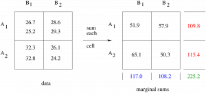
Beginning with the data on the left, sum each cell to give the numbers on the right. In summing each cell you are computing the terms $\sum_{k=1}^{n} x_{i,j,k} = \sum_{k=1}^{2} x_{i,j,k}$ , $1 \leq i,j \leq 2$ in the sum of squares equations on page 234. (Note that these sums are $n$ times the means, $\overline{x}_{i,j }$ , of the cells, which is what the two-way ANOVA compares: $\sum_{k=1}^{n} x_{i,j,k} = n \overline{x}_{i,j}$ .) Next, compute the marginal sums, the sums of the rows, on the far right, and the sums of the columns, on the bottom. Then compute the grand sum, the sum of everything, which is the the sum of the marginal sums on the right which equals the sums on the bottoms (which should be equal — a check). The marginal sums show up in the second inner brackets in the sums of squares formula. Notice that the sums of the rows collapse the design across $B$ to give a one-way ANOVA for $A$ (main effect of $A$ ) and the sums of the columns collapse the design across $A$ to give a one-way ANOVA for $B$ (main effect of $B$ ). With the marginal sums we compute:

$C = \frac{1}{N} \left( \sum \sum \sum x_{i,j,k} \right)^{2} = \frac{{225.2}^{2}}{8} = 6339.38$

$\begin{eqnarray*} \mbox{SS}_{T} & = & \sum \sum \sum x_{i,j,k}^{2} - C \mbox{\ \ \ (This one's not from the marginal sums.)}\\ & = & (26.7^{2} + 25.2^{2} + 28.6^{2} + 29.3^{2} + 32.3^{2} + 32.8^{2} + 26.1^{2} + 24.2^{2}) - 6339.38 \\ & = & 6410.36 - 6339.38 \\ & = & 70.98 \end{eqnarray*}$

$\begin{eqnarray*} \mbox{SS}_{A} & = & \frac{1}{bn} \sum_{i=1}^{a} \left( \sum_{j=1}^{b} \left( \sum_{k=1}^{n} x_{i,j,k} \right) \right)^{2} - C \\ & = & \frac{1}{(2)(2)} \left[ ({109.8})^{2} + ({115.4})^{2} \right] - 6339.38 \\ & = & 6343.30 - 6339.38 \\ & = & 3.92 \end{eqnarray*}$

$\begin{eqnarray*} \mbox{SS}_{B} & = & \frac{1}{an} \sum_{j=1}^{b} \left( \sum_{i=1}^{a} \left( \sum_{k=1}^{n} x_{i,j,k} \right) \right)^{2} - C \\ & = & \frac{1}{(2)(2)} \left[ ({117.0})^{2} + ({108.2})^{2} \right] - 6339.38 \\ & = & 6349.06 - 6339.38 \\ & = & 9.68 \end{eqnarray*}$

$\begin{eqnarray*} \mbox{SS}_{A \times B} & = & \frac{1}{n} \left( \sum \sum \left( \sum x_{i,j,k} \right)^{2} \right) - C - \mbox{SS}_{A} - \mbox{SS}_{B} \mbox{\ (No marginal sums.)} \\ & = & \frac{1}{2} \left( 51.9^{2} + 57.9^{2} + 65.1^{2} + 50.3^{2} \right) - 6339.38 - 3.92 - 9.68 \\ & = & 6407.06 - 6339.38 - 3.93 - 9.68 \\ & = & 54.08 \end{eqnarray*}$

$\begin{eqnarray*} \mbox{SS}_{W} & = & \mbox{SS}_{T} - \mbox{SS}_{A} - \mbox{SS}_{B} - \mbox{SS}_{A \times B} \\ & = & 70.89 - 3.92 - 9.68 - 54.08 \\ & = & 3.30 \end{eqnarray*}$

There. Now the sums of squares are ready for computing the test statistics. At this point you can start making your ANOVA table to keep track of your calculations. Here we’ll see the ANOVA table at the last step.

1. Hypotheses.

$\begin{eqnarray*} H_{0} &:& \mbox{No main effect of $A$. (Changing gas type doesn't change mileage.)} \\ H_{1} &:& \mbox{Main effect of $A$.}\\ \\ H_{0} &:& \mbox{No main effect of $B$. (Changing auto type doesn't change mileage.)} \\ H_{1} &:& \mbox{Main effect of $B$.}\\ \\ H_{0} &:& \mbox{No interaction $A \times B$.} \\ H_{1} &:& \mbox{Interaction $A \times B$. (The effect of gas type on mileage depends on auto type.)} \end{eqnarray*}$

2. Critical statistics.

There are three of them, one for each hypothesis pair. Use the F Distribution Table with the $\alpha$ labelling the table equal to the test $\alpha = 0.05$ since there are no such things as one and two tailed tests for ANOVA. From the F Distribution Table find:

For $A$ :

$\begin{eqnarray*} \nu_{1} & = & a-1=2-1 = 1 \mbox{\ (d.f.N)}\\ \nu_{2} & = & ab(n-1) = (2)(2)(2-1) = 4 \mbox{\ (d.f.D.)}\\ F_{\mbox{crit}} & = & 7.71 \end{eqnarray*}$

For $B$ :

$\begin{eqnarray*} \nu_{1} & = & b-1=2-1 = 1 \mbox{\ (d.f.N)}\\ \nu_{2} & = & ab(n-1) = (2)(2)(2-1) = 4 \mbox{\ (d.f.D.)}\\ F_{\mbox{crit}} & = & 7.71\\ \end{eqnarray*}$

For $A \times B$ :

$\begin{eqnarray*} \nu_{1} & = & (a-1)(b-1)=(2-1)(2-1) = 1 \mbox{\ (d.f.N)}\\ \nu_{2} & = & ab(n-1) = (2)(2)(2-1) = 4 \mbox{\ (d.f.D.)}\\ F_{\mbox{crit}} & = & 7.71 \end{eqnarray*}$

The critical statistics are all the same for a $2 \times 2$ ANOVA ( $\nu_{1} = 1$ for all the hypotheses pairs — essentially three $t$ -tests because $t_{\nu}^{2} = F_{1,\nu}$ ). For bigger designs, the critical statistics will, in general, be different for each hypothesis pair.

3. Test statistics.

Use the sums of squares to compute:

$\mbox{MS}_{A} = \frac{\mbox{SS}_{A}}{a-1} = \frac{3.920}{2-1} = 3.920$

$\mbox{MS}_{B} = \frac{\mbox{SS}_{B}}{b-1} = \frac{9.680}{2-1} = 9.680$

$\mbox{MS}_{A \times B} = \frac{\mbox{SS}_{A \times B}}{(a-1)(b-1)} = \frac{54.080}{(2-1)(2-1)} = 54.080$

$\mbox{MS}_{W} = \frac{\mbox{SS}_{W}}{ab(n-1)} = \frac{3.300}{4} = 0.825$

$F_{A} = \frac{\mbox{MS}_{A}}{\mbox{MS}_{W}} = \frac{3.920}{0.825} = 4.752$

$F_{B} = \frac{\mbox{MS}_{B}}{\mbox{MS}_{W}} = \frac{9.680}{0.825} = 11.773$

$F_{A \times B} = \frac{\mbox{MS}_{A \times B}}{\mbox{MS}_{W}} = \frac{54.080}{0.825} = 65.552$

4. Decision.

In general, we need three diagrams, but in this case all the critical statistics are the same so we can draw :

So :

For $A$ , do not reject $H_{0}$ , there is no main effect of $A$ .
For $B$ , reject $H_{0}$ , there is a main effect of $B$ .
For $A \times B$ , reject $H_{0}$ , there is an interaction.

5. Interpretation.

Simply put, at $\alpha = 0.05$ there is no effect of gas type (factor $A$ ) on mileage; there is an effect of auto type (factor $B$ ) on gas mileage and; there is an interaction between gas type and mileage, the change in mileage with auto type depends on the gas type used. We’ll look at the profile plot to see if we really understand what this means but first we should complete the ANOVA table :

Source	Sum of Squares	Degrees of Freedom	Mean Square	$F_{\rm test}$	p
$A$ (gas)	3.92	1	3.92	$F_{A}$	$p > 0.05$
$B$ (auto)	9.68	1	9.68	$F_{B}$	$p < 0.05$
$A \times B$	54.08	1	54.08	$F_{A \times B}$	$p < 0.05$
Within (error)	3.30	4	0.825
Totals	70.98	7

To draw the profile plot, we need to do one more data reduction :

So the profile plot (without error bars — but remember the numbers are fuzzy) is :

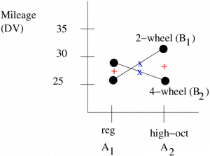
To interpret this fully, remember the rules from previously about collapsing by looking at the midpoints between the two $A$ values and the midpoint of the lines. Here we see that averaged over auto types, it looks like there is no difference in gas mileage between gas type. That conclusion is statistically confirmed by the fact that we found no main effect of factor $A$ , gas — the two + values are not significantly different. The centres of the lines marked by the x are, however, significantly different because we found a main effect of $B$ , auto type. And the nature of the statistically significant interaction is obvious, the gas mileage can go up or down when you change gas types depending on what kind of car you drive. Switching from regular gas to high octane gas will improve your mileage if you drive a 4-wheel drive car but the mileage will get worse if you drive a 2-wheel drive car.

▢

You will see bigger designs than a $2 \times 2$ . Collapsing across $A$ or $B$ in those larger designs to get to one-way ANOVAs is conceptually straightforward. The interaction is trickier, but the idea of an interaction existing when there are statistically non-parallel lines still holds. The $2 \times 2$ ANOVA is essentially three $t$ -tests. This makes the $2 \times 2$ ANOVA powerful and easy to interpret. As always, in statistics simpler is more powerful. We will take a brief quantitative look at statistical power in Chapter 13 but qualitatively, simpler is more powerful.

For the single sample $t$ -test the two values of the IV were the population of interest and a hypothetical population representing $H_{0}$ having the mean $k$ . ↵
Population values are used for this illustration. When you plot profile plots like this you will use sample means. ↵
Remember that "significant" means "reject $H_{0}$ ". ↵
Remember the counting rule! ↵
If the cell sizes, $n_{i,j}$ , are all the same then the average is exactly halfway between the dots. ↵
For equal cell sizes. For unequal cell sizes the x will still be somewhere along the line. ↵
Of course, if you're using SPSS you don't need to restrict yourself to a balanced design. SPSS knows the generic SS formulae. ↵

License

Icon for the Creative Commons Attribution-NonCommercial-ShareAlike 4.0 International License

Introduction to Applied Statistics for Psychology Students Copyright © 2022 by Gordon E. Sarty is licensed under a Creative Commons Attribution-NonCommercial-ShareAlike 4.0 International License, except where otherwise noted.

License

Share This Book