If is rejected in a one-way ANOVA, you will frequently want to know where the differences in the means are. For example if we tested and rejected in a one-way ANOVA then we will want to know if or , etc.

To see which means are different after doing an ANOVA we could just compare all possible combinations of pairs using -tests. But such an approach is no good because the assumed type I error rates, , associated with the -tests would be wrong. The rate would be higher because in making such multiple comparisons you incur a greater chance of making an error.

So we need to correct our test statistic and/or the corresponding value when we do such multiple comparisons. We will cover two such multiple comparison approaches in detail :

1. Scheffé test
2. Tukey test

and we will look at the Bonferroni approach.

Doing multiple comparisons after an ANOVA is known as post hoc testing. It is the traditional approach for comparing several means. The opening “omnibus” ANOVA lets you know if there are any differences at all. If you fail to reject the ANOVA then you are done. Only when you reject do you put in the effort of comparing means pairwise. This traditional approach, designed to minimize the necessary calculations, is not the only way to compare multiple means. The other approach is to forget about the ANOVA and then use -tests to compare means pairwise on in combinations^[1] of means until you use up the degrees of freedom in the dataset. Here we will stick with the traditional approach.

12.2.1 Scheffé test

The test statistic for the Scheffé test is

Note that is basically a quantity (recall that ) but with a pooled estimate of the common population variance given by the value of from the ANOVA. In other words uses information from all of the data to estimate instead of from just groups and as a -test would (see Equation 10.5). Note that the Scheffé test does not require equal group sizes .

The critical statistic is a modification of the critical statistic from the ANOVA is

where and are the ANOVA degrees of freedom. The critical statistic is the same for all pairwise comparisons regardless of the sample sizes, and , of the pair of groups being compared.

Example 12.2 : The ANOVA of Example 12.1 found that at least one of the three means was different from the others. Use the Scheffé test to find the significant differences between the means. There has to be at least one.

Solution :

0. Data reduction.

Collect the necessary information from the omnibus ANOVA. We’ll need:

1. Hypotheses.

There are 3 hypotheses pairs to test :

2. Critical statistic.

One value for all three hypothesis tests:

3. Test statistic.

There are three of them:

vs. :

vs. :

vs. :

4. Decision.

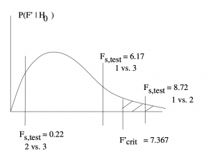
For vs. , reject . For vs. , do not reject . For vs. , do not reject .

5. Interpretation.

The results of the Scheffé test at conclude that only the mean numbers of interchange employees between toll roads 1 and 2 are significantly different.

▢

12.2.2 Tukey Test

The test statistic for the Tukey test is

where, again, is from the omnibus ANOVA, is the mean of group and we must have equal sample sizes for all groups: for all . There is a Tukey test statistic for unequal , and it is used by SPSS, but we won’t cover that here.

The critical statistic, , comes from a table of critical values from a new distribution called the distribution. The critical values are tabulated in the Tukey Test Critical Values Table. To use this table, you need two numbers going in :

1. = number of groups
2. = degrees of freedom for

Reject when . In this case we don’t have a picture of the distribution handy (although it is basically the absolute value of ), so we just use the rule similar to how we use the -value.

Example 12.3 : Repeat Example 12.2 using the Tukey test instead of the Scheffé test.

Solution : 0. Data Reduction.

We use the same data from the omnibus ANOVA :

1. Hypotheses.

The 3 hypotheses pairs to test are the same :

2. Critical statistic.

Use the Tukey Test Critical Values Table. Go into the table with

• Number of groups = .
• .

and to find

3. Test statistic.

Again, there are three of them :

vs. :

vs. :

vs. :

4. Decision.

Reject when . This only happens for one hypothesis pair : For vs. , reject . For vs. , do not reject . For vs. , do not reject .

5. Interpretation.

The results of the Tukey test at conclude that only the mean numbers of interchange employees between toll roads 1 and 2 are significantly different. (Same result as the Scheff test. Usually this happens but when it doesn’t, you need to use some kind of non-mathematical judgement.)

12.2.3 Bonferroni correction

A more conservative (less power) approach to multiple comparisons (post hoc testing) is to use Bonferroni’s method. The fundamental idea of the Bonferroni correction is to add the probabilities of making individual type I errors to get an overall type I error rate.
Implementing the idea is simple. Do a bunch of -tests and multiply the -value by a correction factor . There are a number of ways to choose (you will have to dig to find out which method SPSS uses). The easiest (and most conservative) is to set equal to the number of pairwise comparisons done. So if you have groups then is given by the binomial coefficient:

Another way is to look at the total degrees of freedom, , associated with the pairwise -tests and compare it to the total degrees of freedom in the data, (or one could argue ), to come up with

Since there is some ambiguity as to what we should use for , we will not do Bonferroni post hoc testing by hand. However, be able to recognize Bonferroni results in SPSS, treating the value of as an SPSS blackbox parameter.