
9. Hypothesis Testing
9.4 z-Test for Proportions
The possible hypothesis pairs are :
| Two-tailed Test | Right-tailed Test | Left-tailed Test |
 |
 |
 |
 |
 |
 |
The steps in hypothesis testing for proportions are the same as hypothesis testing for means. Even the generic test statistic formula is the similar :
![\[\mbox{test value }=\frac{\mbox{(observed value)-(expected $H_0$ value)}}{\mbox{standard error}}.\]](https://openpress.usask.ca/app/uploads/quicklatex/quicklatex.com-a0048b07ed4e2d03ce48aec49d35b8ab_l3.png "Rendered by QuickLaTeX.com")
but now the observed and expected values are proportions,  and
and  respectively. The standard error in this case is
![\[\sqrt{\frac{pq}{n}} = \frac{\sigma_{binomial}}{n} = \frac{\sqrt{npq}}{n}\]](https://openpress.usask.ca/app/uploads/quicklatex/quicklatex.com-0d1e207a3566515d91c86f489d13b7cc_l3.png "Rendered by QuickLaTeX.com")
Using this information with the generic form, which mimics a  test statistic, the proportions test statistic is
![\[z_{test} = \frac{\hat{p}-p}{ \sqrt{\frac{pq}{n}}}\]](https://openpress.usask.ca/app/uploads/quicklatex/quicklatex.com-34f64be8d9b9597bc45fb06d40dea599_l3.png "Rendered by QuickLaTeX.com")
where is the number  which appears in the
  hypothesis statement (see table above). This test statistic is valid only if
  and
and  (so that the normal distribution provides a good approximation for the relevant binomial distribution). But, even though the test statistic can be moulded into the generic form, the proportions test statistic comes from the sampling theory given by the binomial distributions and not from any distribution that has a standard error {\em per se}. The normal distribution with
  and
and  (remember those binomial distribution formulae?)
  -transformed to a -distribution with mean 0 and standard deviation 1 gives the test statistic formula. See the discussion in Section 8.4.
Example 9.5 : An attorney claims that more than 25 of all lawyers advertise. A sample of 200 lawyers in a certain city showed that 63 had used some form of advertising. At
  , is there enough evidence to support the attorney’s claim?
Solution :
1. Hypotheses.
 ,
,  (claim)
2. Critical statistic.
Using the t Distribution Table (last line) for a one tailed test at we find 
3. Test statistic.
![\[z_{\rm test} = \frac{\hat{p} - p}{\sqrt{\frac{pq}{n}}}\]](https://openpress.usask.ca/app/uploads/quicklatex/quicklatex.com-3ba0ece5fa0323490001c0fbc55cdcdf_l3.png "Rendered by QuickLaTeX.com")
So using
![\[\hat{p} = \frac{63}{200} = 0.315 \hspace{.25in} p = 0.25\]](https://openpress.usask.ca/app/uploads/quicklatex/quicklatex.com-99886289419486defeebf13166e8d0d4_l3.png "Rendered by QuickLaTeX.com")
![\[q = 1 - 0.25 = 0.75 \hspace{.25in} n = 200\]](https://openpress.usask.ca/app/uploads/quicklatex/quicklatex.com-de53635659fe23ab2190c5bb9dbaad37_l3.png "Rendered by QuickLaTeX.com")
find
![\[z_{\rm test} = \frac{0.35 - 0.25}{\sqrt{\frac{(0.25)(0.75)}{200}}} = 2.12.\]](https://openpress.usask.ca/app/uploads/quicklatex/quicklatex.com-04c9085c10efcca11bafa9e08a3622f9_l3.png "Rendered by QuickLaTeX.com")
We can also find the value along with the critical statistic. (See the picture for the next step.) Use the Standard Normal Distribution Table to find

4. Decision.
Refer to the diagram in Figure 9.4. It shows  in the rejection region. So we reject .
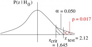
We come, of course, to the same decision by considering the -value :
![\[ (p = 0.017) < (\alpha = 0.5) \]](https://openpress.usask.ca/app/uploads/quicklatex/quicklatex.com-5450dcd08e53ff9b4f477ff5159f0238_l3.png "Rendered by QuickLaTeX.com")
5. Interpretation.
There is enough evidence, using a -test at , to support the claim that more than  of the lawyers use some form of advertising.
▢
