
7. The Central Limit Theorem
7.2 The Central Limit Theorem
Now we come to the very important central limit theorem. First, let’s introduce it intuitively as a process :
- Suppose you have a large population (in theory infinite) with mean
 and standard deviation
  (and any old shape).
 - Suppose you have a large sample, size
 , of values from that population. (In practise we will see that
  is large.) Take the mean,
  , of that sample. Put the sample back into the population[1]
 - Randomly pick another sample of size . Compute the mean of the new sample,
 . Return the sample to the population..
 - Repeat step 3 an infinite number of times and build up your collection of sample means
 .
. - Then[2] the distribution of the sample means will be normal will have a mean equal to the population mean, , and will have a standard deviation of
![\[ \sigma_{\overline{x}} = \frac{\sigma}{\sqrt{n}} \]](https://openpress.usask.ca/app/uploads/quicklatex/quicklatex.com-5ecd1557f673ed549f6bc9836e3bdabb_l3.png "Rendered by QuickLaTeX.com")
where
is the population’s standard deviation.  is known as the standard error of the mean.
Now let’s visualize this same process using pictures :
- Take a sample of size from the population and compute the mean
 (see Figure 7.2a).

- Put them back and take more data points.
- Do this over and over to get a bunch of values for . Those values for will be distributed as shown in Figure 7.2b.
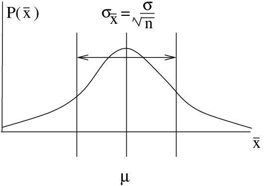
The central limit theorem is our fundamental sampling theory. It tells us the if we know what the mean and standard deviation of a population[3] are then we can assign the probabilities of getting a certain mean in a randomly selected sample from that population via a normal distribution of sample means that has the same mean as the population and a standard deviation equal to the standard error of the mean.
To apply this central limit theorem sampling theory we will need to compute areas  under the normal distribution of means. In order to do that, so we can use the Standard Normal Distribution Table, we need to convert the values
  to a standard normal
  using the -tranformation as usual:
  . So, for the distribution of sample means the appropriate -transformation is :
![\[ z = \frac{\overline{x} - \mu}{\sigma\sqrt{n}}\]](https://openpress.usask.ca/app/uploads/quicklatex/quicklatex.com-662ef4cff8775eec507898d0feb0f9c1_l3.png "Rendered by QuickLaTeX.com")
Example 7.1 : Assume that we know, say from SGI’s database, that the mean age of registered cars is  months and that the population standard deviation of the cars is
  months. We make no assumption about the shape of the population distribution. Then, what is the answer to the following sampling theory question: What is the probability that the mean age is between 90 and 100 months in a sample of 36 cars?
Solution : The central limit theorem tells us that sample means will be distributed as shown in Figure 7.3.
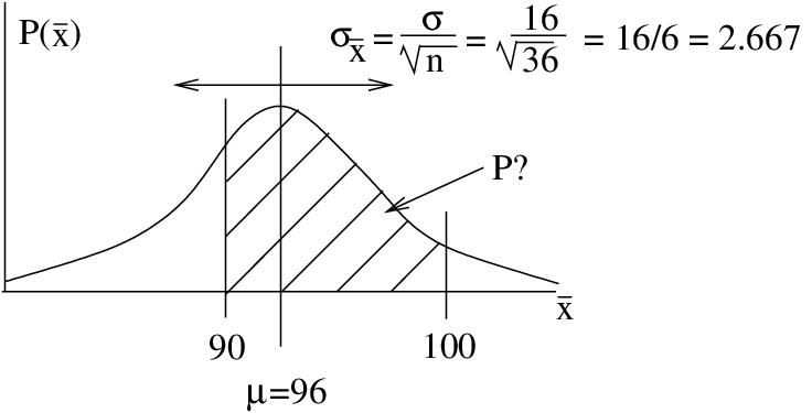
Convert 90 and 100 to -scores as usual:

Then, the required probability using the Standard Normal Distribution Table is

▢
- This is redundant since the population is infinite, but for conceptual purposes imagine that you return the items to the population. ↵
- More precisely, the distribution of sample means asymptotically approaches a normal distribution as
 . But 30 is close enough to infinity for most practical purposes and the statistical inferential tests that we will study will assume that the distribution of sample means will be normal. ↵
 - In hypothesis testing we know what the mean of the population in the null hypothesis is. ↵
