
6. Percentiles and Quartiles
6.1 Discrete Data Percentiles and Quartiles
Before we get into how to calculate percentile in a data set, note that we can see percentiles directly on a cumulative frequency plot, see Figure 6.2.
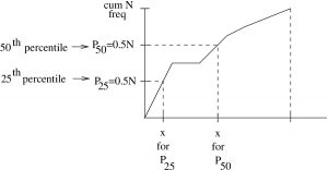
 axis. If you have a newborn baby and take it to the doctor for their first check up, they will measure the baby’s head circumference and tell you the baby’s head size percentile by looking at such a chart. The doctor’s chart will be based on an accumulation of a very large number of essentially population data. Cumulative frequency graphs, or more exactly cumulative probability graphs, can be made for continuous distributions like the normal distribution. The resulting function is the Cumulative Distribution Function, or CDF, and is, for example, P(z) represents the z-distribution then CDF
  . We will see this CDF in SPSS.
Computing percentile positions of discrete data. Let  be the ordered position of a data set of
  data points, then we define the percentile position of
  to be
to be
(6.1) 
This formula has the property that  and
and  . It is what we will use as a percentile formula but it is not the only one. Look at Figure 6.1. The way the histogram there is shaded the formula would be
  which would have the property that
  and
and  . There are other, not necessarily wrong, ways to define the percentile position of discrete data but we will use Equation 6.1.
If you want to find the position, , of the data point corresponding to a given percentile  then compute
(6.2) ![\begin{equation*} i = \left[ \frac{P \times (n-1)}{100} \right] + 1. \end{equation*}](https://openpress.usask.ca/app/uploads/quicklatex/quicklatex.com-d9bb869212d32ea89e92f4fb09b77614_l3.png "Rendered by QuickLaTeX.com")
Equation (6.2) is derived by solving Equation (6.1) for . Note that Equation (6.2) gives the position of the data point , not its value. To clarify that, let’s look at an example.
Example 6.1 : Consider the dataset given below. Data would originally be given as the numbers in the first line. So the first step in answering any question about percentiles is to order the data, the same as what you need to to to determine the median of a dataset. Once the data are ordered, then you may assign a position number to each data point as shown in the third line.
| original data | 18 | 15 | 12 | 6 | 8 | 2 | 3 | 5 | 20 | 10 |
| ordered data | 2 | 3 | 5 | 6 | 8 | 10 | 12 | 15 | 18 | 20 |
|
1 | 2 | 3 | 4 | 5 | 6 | 7 | 8 | 9 | 10 |
 |
||||||||||
Q : What is the percentile rank of  ?
?
A :  so
so  percentile.
Q : What is the value corresponding to the  percentile,
  ?
?
A : ![i = \left[ \frac{P \times (n-1)}{100} \right] +1 =\left[ \frac{(25) \times (10-1)}{100}\right] +1 = \left[ \frac{25 \times 9}{100}\right] + 1 = 2.25 + 1 = 3.25](https://openpress.usask.ca/app/uploads/quicklatex/quicklatex.com-1976877ad8ee89566389f23d650afaaa_l3.png "Rendered by QuickLaTeX.com")
The closest is 3 and  . We can write
  .
.
▢
Decile :
 The decile of data value in the ordered position is defined as
![\[ D(x_i) = \frac{P(x_i)}{10} \hspace{1in} 0 \leq D(x_{i}) \leq 10 \]](https://openpress.usask.ca/app/uploads/quicklatex/quicklatex.com-88a6775a52018240150631d46c8e3425_l3.png "Rendered by QuickLaTeX.com")
We will not make much use of decile except to see that quartile is defined in the same way.
Quartile :
 The quartile of data value
  in the ordered position 1.
(6.3) 
Notation : (This notation also applies to and  .) We write :
 &=&
&=&  quartile
 & = &
& = &  quartile
 & = &
& = &  quartile
 & = &
& = &  quartile
 & = &
& = &  quartile
Quartiles are useful because we do not have to compute percentile first and then divide by 25 as given by Equation (6.3). Instead, we can use the following handy tricks after ordering our data:

Example 6.2 : Example with an even number of data points. With the data in order, first find the median, then the medians of the two halves of the dataset :
![\[5 \hspace{.25in} 6 \hspace{.25in} 12 \hspace{.25in} 13 \hspace{.25in} 15 \hspace{.25in} 18 \hspace{.25in} 22 \hspace{.25in} 50\]](https://openpress.usask.ca/app/uploads/quicklatex/quicklatex.com-8c2a94eb58322a44e820a0a5e7ffb62f_l3.png "Rendered by QuickLaTeX.com")


▢
Example 6.3 : Example with an even number of data points. With the data in order, first find the median, then the medians of the two halves of the dataset :
![\[2 \hspace{.25in} 5 \hspace{.25in} 11 \hspace{.25in} 14 \hspace{.25in} 18 \hspace{.25in} 25 \hspace{.25in} 35\]](https://openpress.usask.ca/app/uploads/quicklatex/quicklatex.com-f0cccf8b22df5916a9cd0199c4166bb0_l3.png "Rendered by QuickLaTeX.com")


▢
