
10. Comparing Two Population Means
10.3 Difference between Two Variances – the F Distributions
Here we have to assume that the two populations (as opposed to sample mean distributions) have a distribution that is almost normal as shown in Figure 10.2.
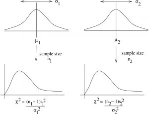
Figure 10.2: Two normal populations lead to two  distributions that represent distributions of sample variances. The
  distribution results when you build up a distribution of the ratio of the two sample values.
The ratio  follows an -distribution if
  . That distribution has two degrees of freedom: one for the numerator (d.f.N. or
  ) and one for the denominator (d.f.D. or
  ). So we denote the distribution more specifically as
  . For the case of Figure 10.2,
  and
and  . The ratio, in general is the result of the following stochastic process. Let
  be random variable produced by a stochastic process with a
  distribution and let
  be random variable produced by a stochastic process with a
  distribution. Then the random variable
  will, by definition, have a distribution.
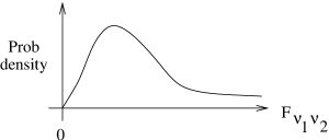
The exact shape of the  distribution depends on the choice of
  and
and  , But it roughly looks like a
  distribution as shown in Figure 10.3.
 distribution.
 and  are related :
![\[F_{1,\nu} = t^{2}_{\nu}\]](https://openpress.usask.ca/app/uploads/quicklatex/quicklatex.com-ee5f0a1e26c1b69034f5084cd4cea1bd_l3.png "Rendered by QuickLaTeX.com")
so the statistic can be viewed as a special case of the statistic.
For comparing variances, we are interested in the follow hypotheses pairs :
| Right-tailed | Left-tailed | Two-tailed |
 |
 |
 |
 |
 |
 |
We’ll always compare variances ( ) and not standard deviations (
 ) to keep life simple.
The test statistic is
![\[ F_{\rm test} = F_{\nu_1, \nu_2} = \frac{s^{2}_{1}}{s^{2}_{2}} \]](https://openpress.usask.ca/app/uploads/quicklatex/quicklatex.com-37f19ee6bebbcb8519703c7df58699a1_l3.png "Rendered by QuickLaTeX.com")
where (for finding the critical statistic),  and
and  .
.
Note that  when
when  , a fact you can use to get a feel for the meaning of this test statistic.
Values for the various critical values are given in the F Distribution Table in the Appendix. We will denote a critical value of with the notation :
![\[F_{\rm crit} = F_{\alpha, \hspace{.1in}\nu_{1}, \hspace{.1in} \nu_2}\]](https://openpress.usask.ca/app/uploads/quicklatex/quicklatex.com-e67b716c4f048bae97f4085cce276088_l3.png "Rendered by QuickLaTeX.com")
Where:
 = Type I error rate
= d.f.N.
= d.f.D.
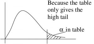
The F Distribution Table gives critical values for small right tail areas only. This means that they are useless for a left-tailed test. But that does not mean we cannot do a left-tail test. A left-tail test is easily converted into a right tail test by switching the assignments of populations 1 and 2. To get the assignments correct in the first place then, always define populations 1 and 2 so that  . Assign population 1 so that it has the largest sample variance. Do this even for a two-tail test because we will have no idea what
  on the left side of the distribution is.
Example 10.3 : Given the following data for smokers and non-smokers (maybe its about some sort of disease occurrence, who cares, let’s focus on dealing with the numbers), test if the population variances are equal or not at  .
.
| Smokers | Nonsmokers |
 |
 |
 |
 |
Note that  so we’re good to go.
Solution :
1. Hypothesis.

2. Critical statistic.
Use the F Distribution Table; it is a bunch of tables labeled by “” that we will designate at  , the table values that signify right tail areas. Since this is a two-tail test, we need
  . Next we need the degrees of freedom:
![\[\mbox{d.f.N.} = \nu_{1} = n_{1} - 1 = 26-1 = 25\]](https://openpress.usask.ca/app/uploads/quicklatex/quicklatex.com-a717a4ff85ed2f607ce0b598a36a043e_l3.png "Rendered by QuickLaTeX.com")
![\[\mbox{d.f.D.} = \nu_{2} = n_{2} - 1 = 18-1 = 17\]](https://openpress.usask.ca/app/uploads/quicklatex/quicklatex.com-e6a75348eeae70738b6cd1ee0084d259_l3.png "Rendered by QuickLaTeX.com")
So the critical statistic is
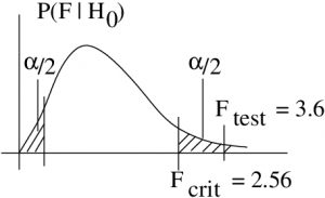
![\[F_{\rm crit} = F_{\alpha/2, \nu_1, \nu_2} = F_{0.05/2, 25, 7} = F_{0.025, 25, 17} = 2.56.\]](https://openpress.usask.ca/app/uploads/quicklatex/quicklatex.com-1b2dd50ba54fc7ad730fdad80a82f1fb_l3.png "Rendered by QuickLaTeX.com")
3. Test statistic.
![\[F_{\nu_1, \nu_2} = \frac{s^2_1}{s^2_2}\]](https://openpress.usask.ca/app/uploads/quicklatex/quicklatex.com-ee568aaf7b85a389ace22d77d991b970_l3.png "Rendered by QuickLaTeX.com")
![\[F_{\rm test} = F_{25, 17} = \frac{36}{10} = 3.6\]](https://openpress.usask.ca/app/uploads/quicklatex/quicklatex.com-6dfc8d85de6b288a26e6b7a12f2015c8_l3.png "Rendered by QuickLaTeX.com")
With this test statistic, we can estimate the  -value using the F Distribution Table. To find , look up all the numbers with d.f.N = 25 and d.f.N = 17 (24
  17 are the closest in the tables so use those) in all the the F Distribution Table and form your own table. For each column in your table record and the value corresponding to the degrees of freedom of interest. Again, corresponds to
  for a two-tailed test. So make a row above the row with
  . (For a one-tailed test, we would put
  .)
.)
|
0.20 0.10 0.05 0.02 0.01 0.10 0.05 0.025 0.01 0.005 |
|
1.84 2.19 2.56 3.08 3.51 3.6 is over here somewhere so  |
Notice how we put an upper limit on because  was larger than all the values in our little table.
Let’s take a graphical look at why we use  in the little table and
  for finding for two tailed tests :
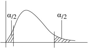
But in a two-tailed test we want split on both sides:
4. Decision.
Reject  . The -value estimate supports this :
![\[ ( p < 0.01) < (\alpha = 0.05) \]](https://openpress.usask.ca/app/uploads/quicklatex/quicklatex.com-401b2b73f94a1a7866da3eba4a06425f_l3.png "Rendered by QuickLaTeX.com")
5. Interpretation.
There is enough evidence to conclude, at with an -test, that the variance of the smoker population is different from the non-smoker population.
▢
