1.1.1 Textbook Layout, * and ** Symbols Explained

This textbook has been designed for use in the statistics classes for psychology I teach at the University of Saskatchewan. It is designed to replace the expensive, and inadequate, texts that have traditionally been used for these classes.

The courses covered by this text are:

1. Univariate Statistics I: Chapters 1 to 10 (Psy 233, undergraduate course)
2. Univariate Statistics II: Chapters 11 to 17 (Psy 234, undergraduate course)
3. Multivariate Statistics: Future project (Psy 807, graduate course)

Since these courses are applied statistics courses, students do not need to understand the derivations of the formulae and procedures. So these aspects, the “cookbook” approach, is what you need to learn to pass the applied statistics courses.

Sections Marked with ** : But, in the sections marked with a ** there are detailed derivations for those who don’t want to believe in magic. Most psychology students will want to skip the ** sections.

Sections Marked with * : Other sections are marked with a *; those sections contain applied statistics material that is not part of the course but is material that an experimental psychology student has a good chance of needing in experimental courses and research projects. (The graduate course Psy 805 is a review of Psy 233/234 with the additional * sections covered — so this text might also be used for Psy 805.)

Psychology students at the University of Saskatchewan are required to learn how to use the statistics program SPSS. So “Lessons” for learning SPSS are included included throughout the text, with RStudio Lessons as an alternative using a different program.

For Univariate Statistics I, the class material is organized in 3 blocks:

• Block 1 is an introduction to the basic tools of statistics and probability — Chapters 1 to 6.
• Block 2 gets you into the ideas of hypothesis testing — Chapter 9.
• Block 3 is material on one- and two-sample -tests — Chapters 9 and 10.

1.1.2 Intro to Univariate Statistics

So, to begin the course material proper, we may identify two “kinds” of statistics:

1. Descriptive Statistics: The presentation, organization and description of data. (Graphs, means, standard deviations, etc.) Block 1 material is primarily about descriptive statistics. Descriptive statistics lead to ideas about probability – we will cover probabilities as given by functions known as the binomial distribution and the normal distribution.
2. Inferential Statistics: The use of probability to infer things about a population from a sample through the use of hypothesis testing. Why do we need inferential statistics? Because it is usually impossible to measure (poll) an entire population.

The goal of Univariate Statistics I is to understand inferential statistics as embodied in the -tests. With blocks 2 and 3 we will build up the background for, and then learn 3 kinds of “-tests” to infer means in populations. To foreshadow, let’s take a look at a simple example. Say we are interested in people’s heights. Let’s look at three situations, corresponding to the three types of -tests we will learn.

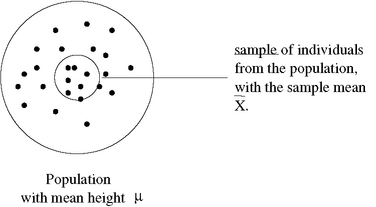
1. One sample -test. The situation is as illustrated in Figure 1.1.

The -test will tell you when you may conclude that:

Here the population could be the height of 10 year old children in Saskatchewan. The quantity is the actual average height of 10 year old kids in Saskatchewan. You could, in principle, measure all the 10 year olds in Saskatchewan but, in practice you can’t. Even if you spent the time finding them all and measuring their heights with a tape measure, they will be growing while you measure them all. It’s generally impossible to measure a population in practice for some reason. Practically, we can only measure a small sample of children from the population. That sample will have a mean that we denote with . The -test is a hypothesis test in which we compare the sample mean to a hypothetical mean and conclude with a probabilistic inference about .

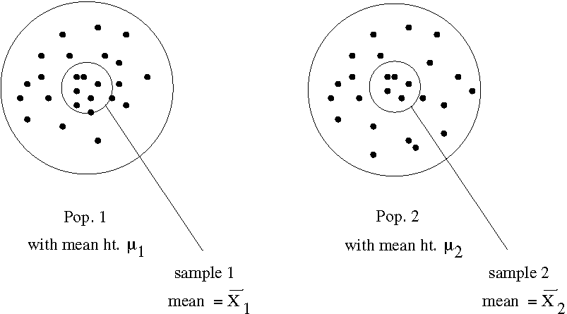
2. Two sample -test. The situation is as illustrated in Figure 1.2.

The t-test will tell you when you can believe that

on the basis that . (The symbol means “approximately equal to”.)

Here the two populations could be 10 year olds (population 1) and 11 year olds (population 2) in Saskatchewan. You might measure the two populations to get some idea about how much 10 year old kids in Saskatchewan grow in one year. The two sample -test will give you information on the difference of the average heights in the population, on the basis of the difference of the means of small samples that you take from each population, .

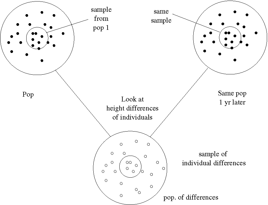
3. Paired -test. The situation is as illustrated in Figure 1.3.

Say we want to know how fast a population grows in 1-year (e.g. pop = 10 year old kids). You can do the two-sample test with two separate populations but if you want to know how the environment affected the growth of the children (maybe you are concerned that they don’t get enough to eat) then the two-sample test is only an approximation. The genetic composition, the natural ability to grow, may be different in the two separate populations. To get at the effect of the environment, without the measurements being confounded by individual differences, we would take a sample of 10 year old kids from the population now and measure their heights. Then we wait a year and measure the height of the same sample of now 11 year old kids. Then we combine the two samples of data into one data sample of differences. The Paired -test will tell you if the average of differences (in heights) is zero or not.