12.3 SPSS Lesson 8: One-way ANOVA

To follow along, load in the Data Set “BoneStrength.sav”:

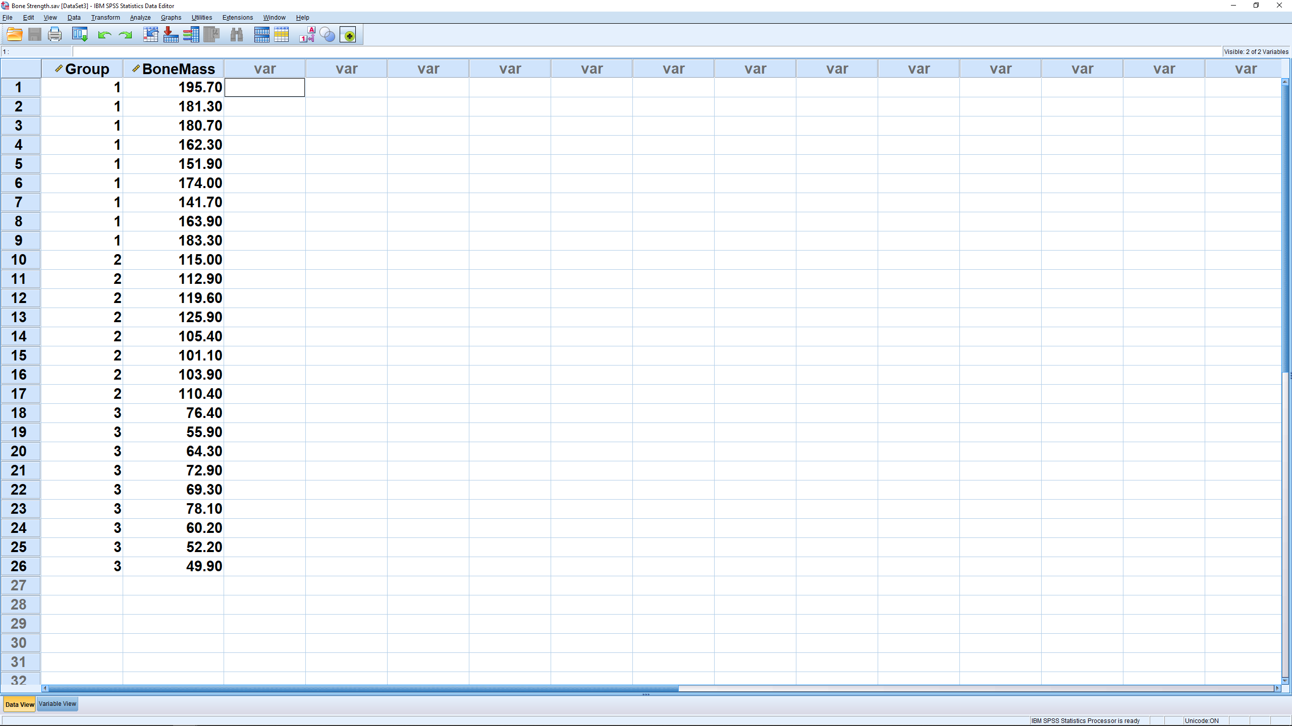
The data format is exactly the same as used for an independent samples -test, except now there are more than two groups in the independent variable, named group in this case. The dependent variable here is diff and we want to test the hypothesis

(12.1)  

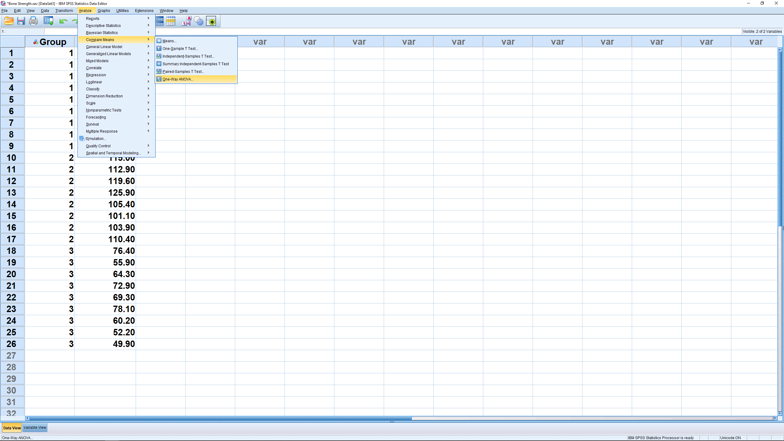
There are two ways to do this in SPSS. We’ll cover each one. The first method is to go through Analyze → Compare means → One-Way ANOVA :

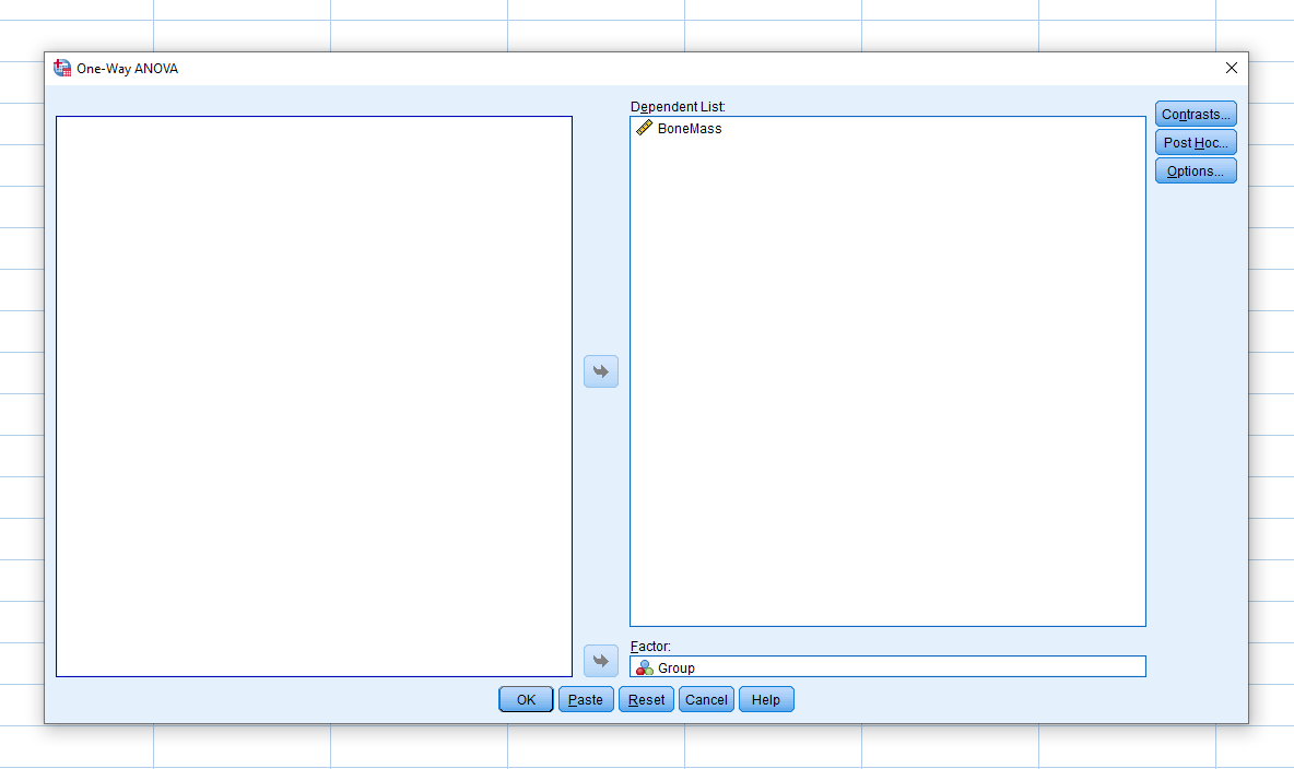
Move the independent variable into the Factor box and the dependent variable into the Dependent List box :

We will ignore the Contrasts menu but the Post Hoc menu is where you set things up for Post Hoc analyses :

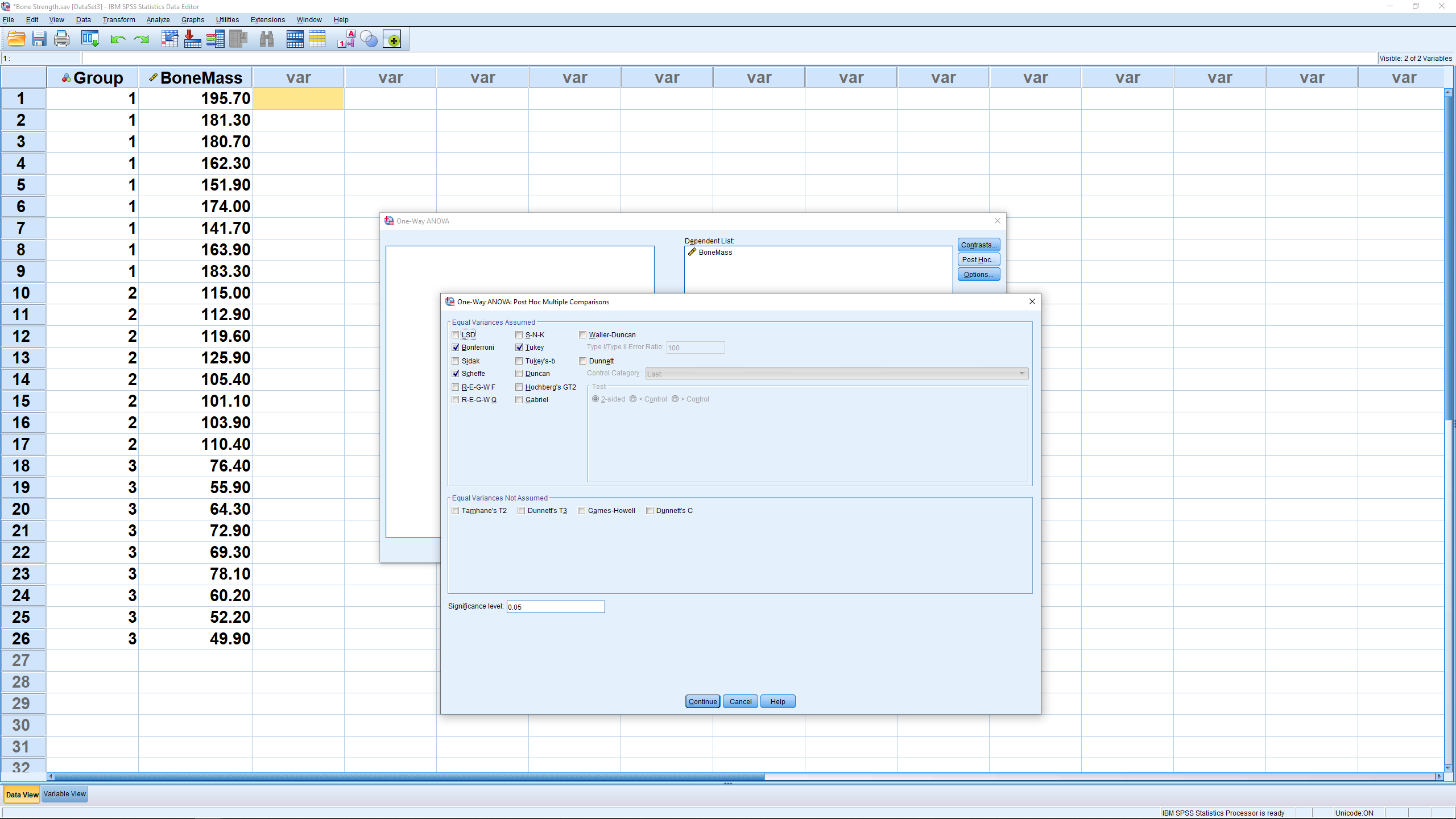
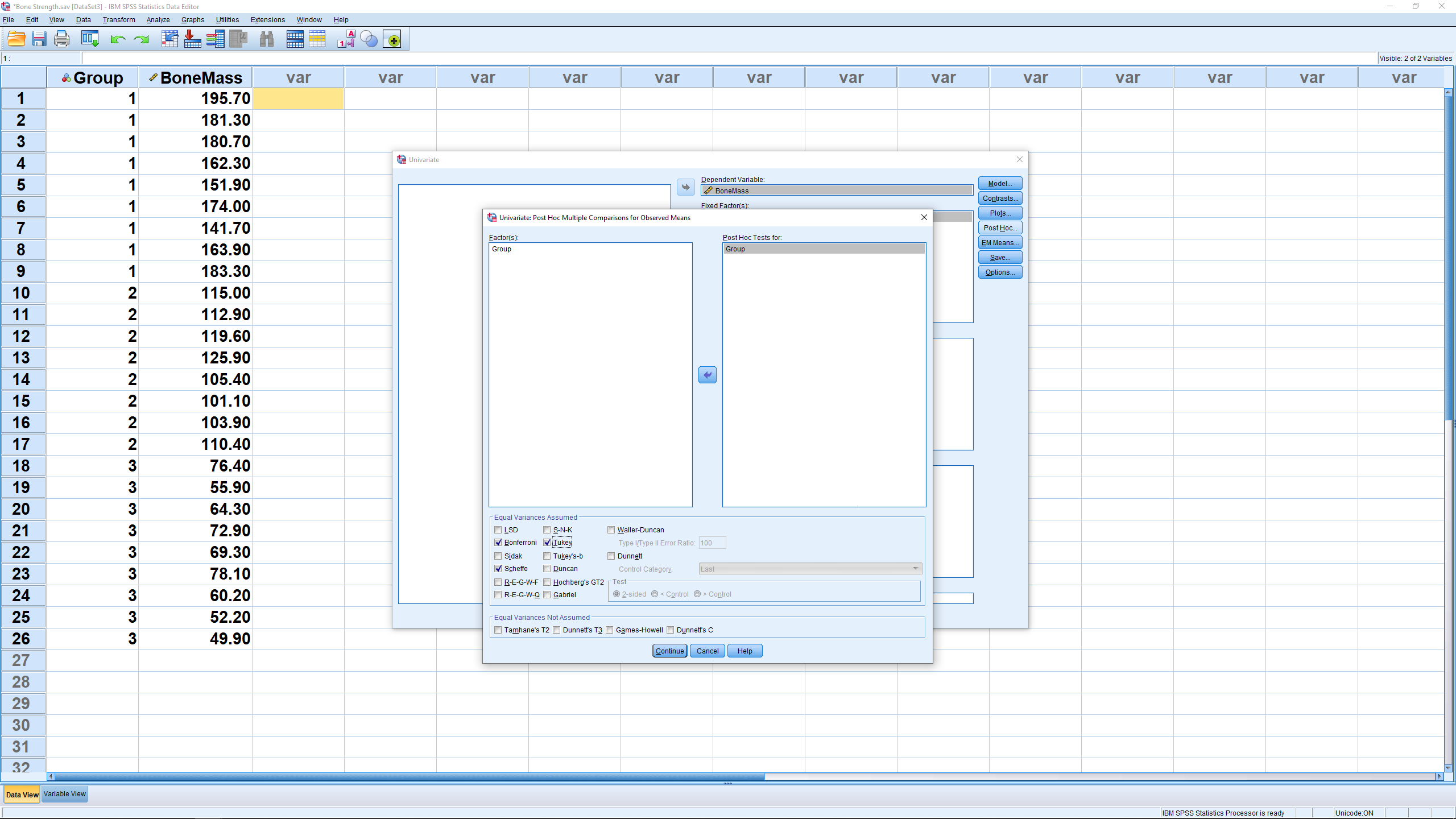
We have checked off Bonferroni, Scheffe and Tukey in the “Equal Variances Assumed” box — we will be assuming homoscedasticity for all our ANOVA work. Hit Continue then OK to get the output :

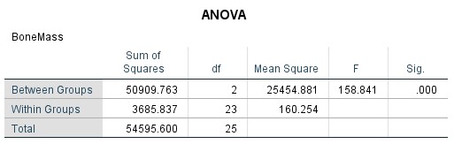
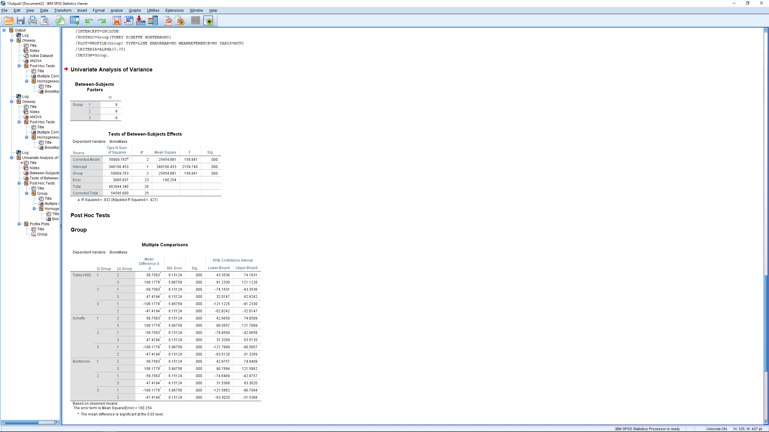
The first table is the ANOVA table. The third column can be obtained from the first two since . The fourth column is, of course, . The Sig.~column gives so we reject .

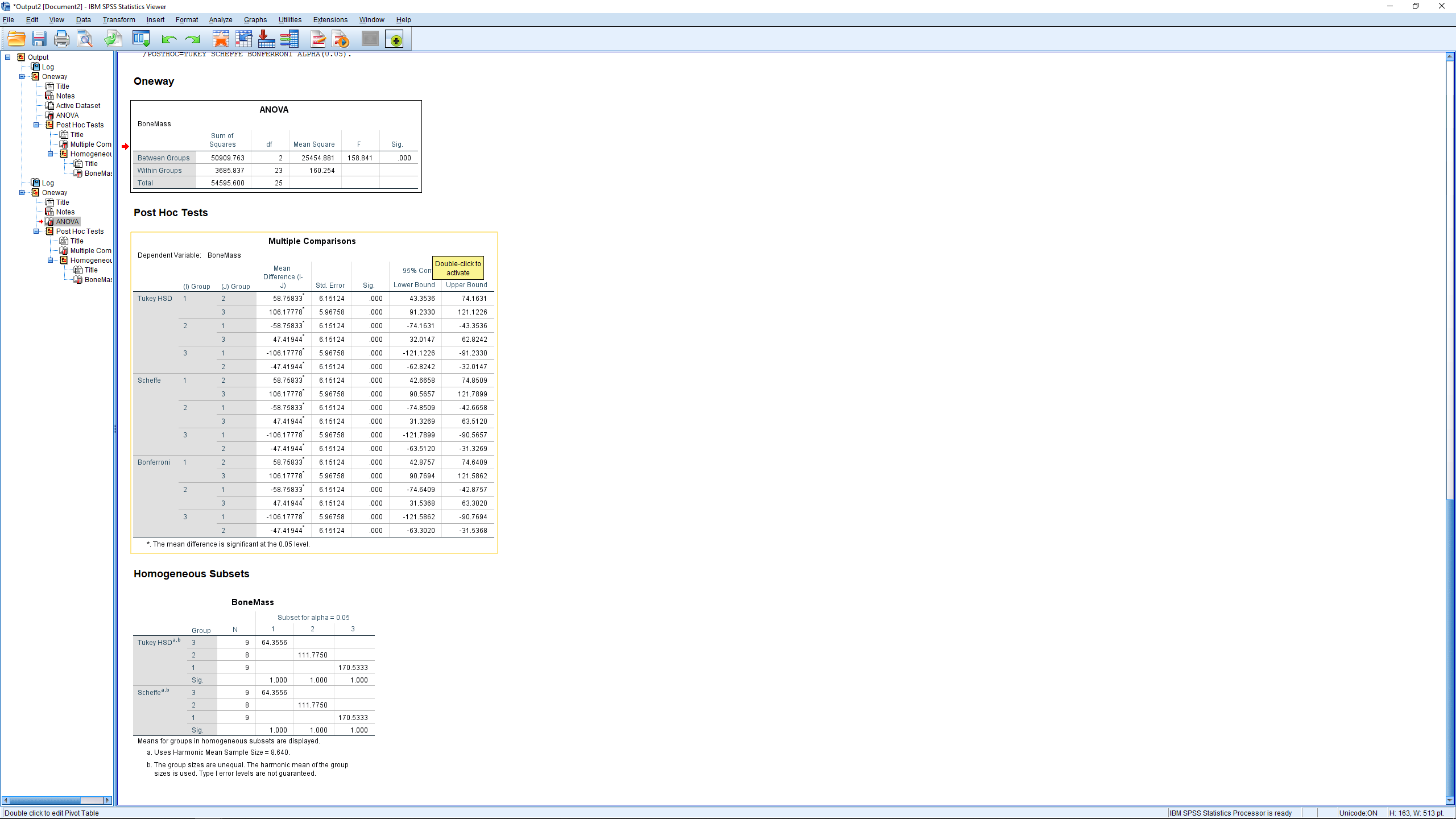
The next table, which is not nonsense since the ANOVA tells us that at least one of the means is different, gives all the pairwise comparisons in a very redundant way. For each test we checked, all three pairs of means are compared — twice (hugely sloppy programming in my opinion). Looking through the table we see that and are significantly different from zero as indicated by the * or as can be seen by looking at the -values. The difference is significantly different from zero. Here all three post hoc methods disagreed. If there is ever a disagreement then you should choose the most conservative result, the one with the lease amount of significant differences.

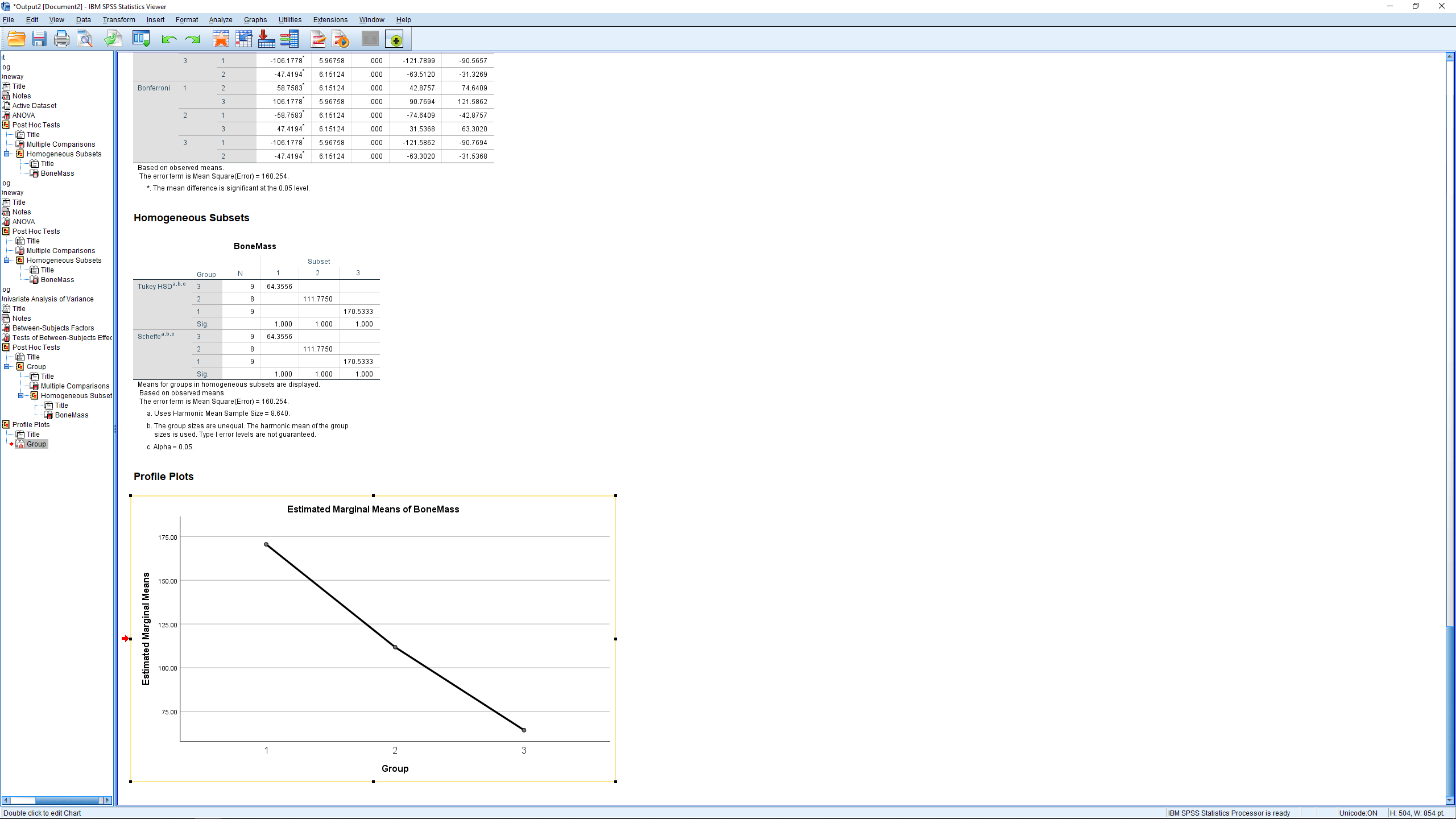
We won’t worry too much about the last table. It merges groups that are not significantly different from each other into “homogeneous subsets”. Here groups 2 and 3 are considered the same and merged into homogeneous subset 1 while group 1 stands on its own as homogeneous subset 2.

The other way of doing a one-way ANOVA is to pick Analyze → General Linear Model → Univariate :

This brings up :

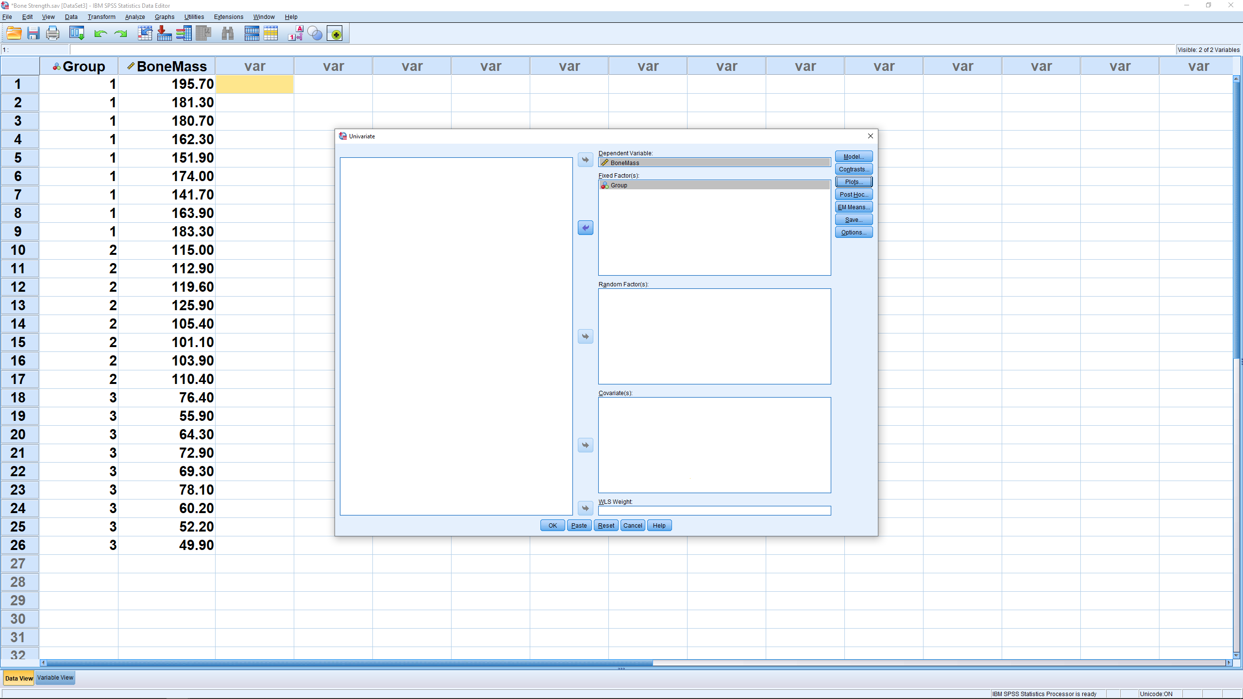
Move the dependent variable into the Dependent Variable box and the independent variable, known as a factor in ANOVA language, into the Fixed Factor box. You will be entering two fixed factors in here when we get to 2-way ANOVA. The Random Factor is for the case where there are multiple populations (factors) and you do not get data from all of them, but only from a random sample of those populations. We will not cover this approach here but you can use it no problem in the future if you have to, it works the same way but the SS formulae are different. The Covariate box is for a method known as ANCOVA (analysis of covariance). We will not cover ANCOVA here, but note that it is a combination of ANOVA and linear regression.

Look at the Model menu and leave the button selected to “Full Factorial” (for one-way ANOVA this is the only choice anyway) and leave the “Include intercept in model” button as selected too. We’ll leave Contrasts as it is too. Open plots and set it up as, by clicking group into “Horizontal Axis” and then clicking Add, so we can get a profile plot :

Finally, open the Post Hoc menu and set it up the same way as we set up the Post Hoc menu above :

Hit Continue the OK to get the output :

The output is pretty much the same as before (the homogeneous subsets is output also but it is not shown here) but the ANOVA table is a little different. In particular there are extra lines in the ANOVA table that you need to learn to ignore. The relevant lines are group (between), Error (within) and “Corrected Total”. When we run this analysis we had the “Include intercept in model” box checked, if we unchecked that box then the ANOVA table will not contain an Intercept line.

The output also contains a profile plot where we can clearly see that the mean for group 1 is different from the other two groups :

We skipped the Save and the Options menu when we set up the test. Take a look at the Save menu. You will see a bunch of essentially descriptive statistics that we won’t worry about here. In the Options menus, though, check off a couple of items, as shown here, and re-run :

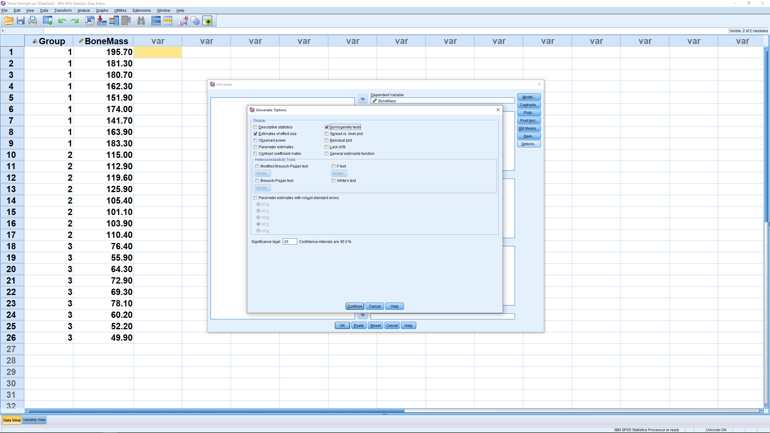
This time you get an additional table for Levine’s test and more information in the ANOVA table :

Levine’s test has so we do not reject the null hypothesis of homosecdasticity between the three groups. This is just a test of assumptions about the sums of squares formulae using in the analysis. The ANOVA table contains a column for the descriptive strength of association. Note that it is the same as R squared.

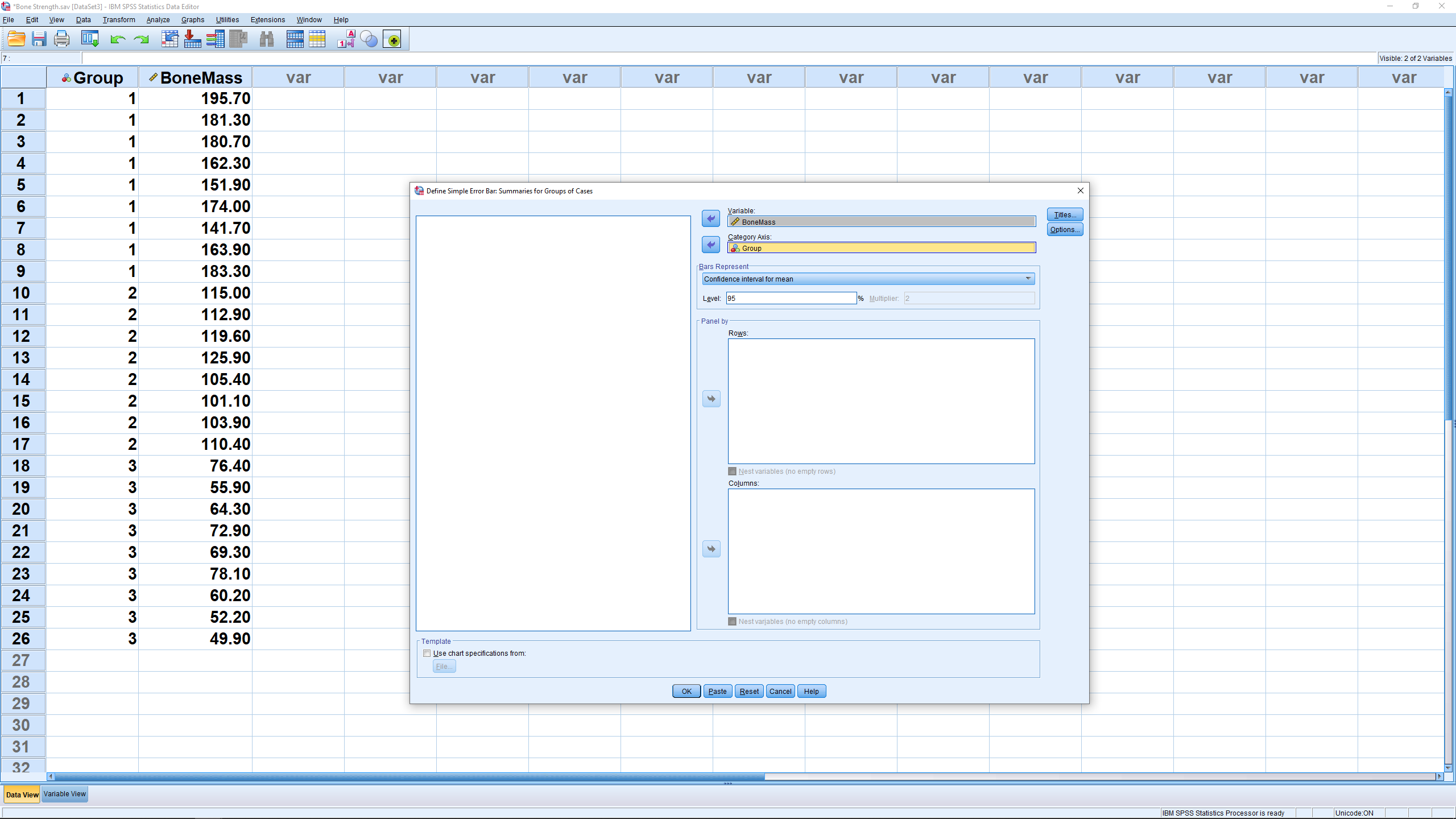
The profile plot produced by the ANOVA analysis can be miss leading if is large. To see the scatter in the data more clearly, we can make profile plots with error bars. Go to Graphs → Legacy Dialogs → Error Bar, leave the default settings at Simple and “Summaries for groups of cases”. Then set up the menu as follows.

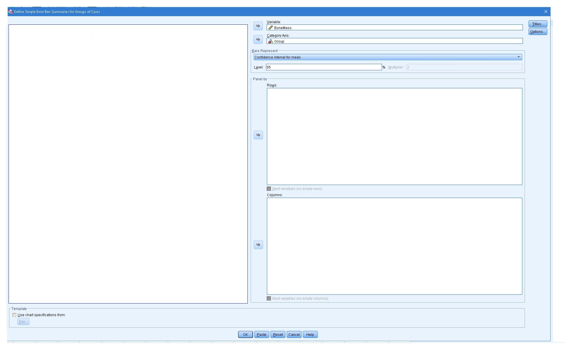
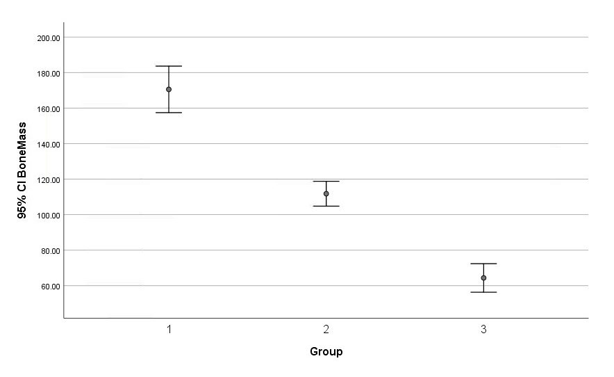
This produces :

Similarly we can produce a boxplot version :

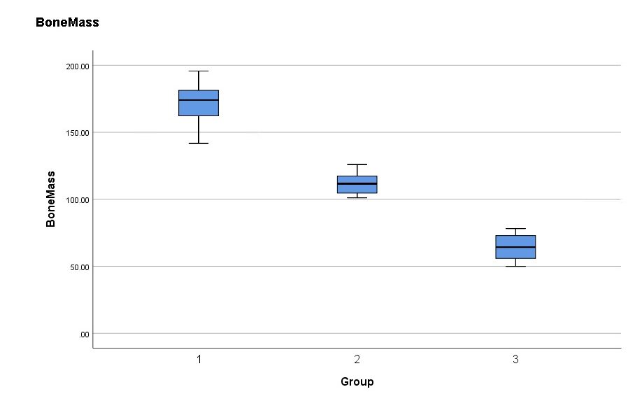
The ANOVA correctly identified the means of all groups as being different. This kind of information can drastically change your interpretation of the results (in this case that group C may not be as effective as the ANOVA indicates).