10.1 Unpaired z-Test

Gordon E. Sarty

10. Comparing Two Population Means

10.1 Unpaired z-Test

We have two populations and two sample sets, one from each population :

Sample Mean

Sample std. dev.

From population 1

$\overline{x}_{1}$

$s_{1}$

From population 2

$\overline{x}_{2}$

$s_{2}$

The population means are $\mu_{1}$ and $\mu_{2}$ and just as with the single population test, there are 3 possible hypothesis tests :

Two Tailed

Right Tailed

Left Tailed

$H_0: \mu_1 = \mu_2$

$H_0: \mu_1 \leq \mu_2$

$H_0: \mu_1 \geq \mu_2$

$H_1: \mu_1 \neq \mu_2$

$H_1: \mu_1 > \mu_2$

$H_1: \mu_1 < \mu_2$

or

$H_0: \mu_1 - \mu_2$ = 0

$H_0: \mu_1 - \mu_2 \leq$

$H_0: \mu_1 - \mu_2 \geq 0$

$H_1: \mu_1 - \mu_2 \neq 0$

$H_1: \mu_1 - \mu_2 > 0$

$H_1: \mu_1 - \mu_2 <0$

In the second row the hypotheses are written in terms of a difference. Irrespective of which way you write the hypotheses, give population 1 priority. Write population 1 first. That way you won’t mess up your signs or your interpretation.

The test statistic to use, in all cases^[1] is

(10.1) $\begin{equation*} z_{\rm test} = \frac{(\bar{x}_1 - \bar{x}_2)}{\sqrt{\frac{s^2_1}{n_1} + \frac{s^2_2}{n_2}}} \end{equation*}$

where $n_{1}$ = sample set size from population 1 and $n_{2}$ = sample set size from population 2. This test statistic is based on a distribution of sample means as shown in Figure 10.1.

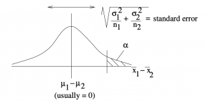
Figure 10.1 : The distribution of the difference of sample means $\bar{x}_{1} - \bar{x}_{2}$ under the null hypothesis $H_{0}: \mu_{1} - \mu_{2} = 0$ . A one-tail example is shown here. The test statistic of Equation 10.1 follows from a $z$ -transformation of this picture.

Example 10.1 : A researcher hypothesizes that the average number of sports colleges offer for males is greater than the average number of sports offered for females. Samples of the number of sports offered to each sex by randomly selected colleges is given here :

Males (pop. 1)

Females (pop. 2)

$n_{1} = 50$

$n_{2} = 50$

$\bar{x}_{1} = 8.6$

$\bar{x}_{2} = 7.9$

$s_{1} = 3.3$

$s_{2} = 3.3$

At $\alpha = 0.10$ is there enough evidence to support the claim?

Solution :

1. Hypotheses.

$H_{0}: \mu_1 \leq \mu_2 \hspace{.5in} H_{1}: \mu_1 > \mu_2 \mbox{ (claim)}$

Note that $\bar{x}_{1} > \bar{x}_{2}$ ( $8.6>7.9$ ) so $H_{1}:\mu_1 > \mu_2$ is true on the face of it. If $H_{1}$ is not true on the face of it then $H_{1}$ is just plain false without the need for any statistical test. With the hypotheses direction set correctly, the question becomes: Is $\bar{x}_{1}$ significantly greater than $\bar{x}_2$ ? The term “statistically significant” corresponds to “reject $H_{0}$ “.

2. Critical statistic.

From the t Distribution Table, one-tailed test at $\alpha = 0.10$ we find

$z_{\rm crit} = 1.282$

Note that $z_{critical}$ is positive because this is a right-tailed test. For left tailed tests make $z_{\rm crit}$ negative. For two-tailed tests you have $\pm z_{\rm crit}$ .

3. Test statistic.

$\begin{eqnarray*} z &=& \frac{(\bar{x}_1 - \bar{x}_2)}{\sqrt{\frac{s^2_1}{n_1} + \frac{s^2_2}{n_2}}} \\ &=& \frac{(8.6 - 7.9)}{\sqrt{\frac{3.3^2}{50} + \frac{3.3^2}{50}}} \\ &=& 1.06 \end{eqnarray*}$

Using the Standard Normal Distribution Table, we can find the $p$ -value. Since $A(z) = A(1.06) = 0.3554$ , $p = 0.05 - 0.3554 = 0.1446$ .

4. Decision.

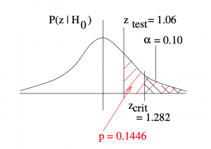
Do not reject $H_{0}$ since $z_{\rm test}$ is not in the rejection region. The $p$ -value reflects this :

$(p = 0.1446) > (\alpha = 0.10)$

5. Interpretation.

There is not enough evidence, at $\alpha = 0.10$ under a $z$ -test, to support the claim that colleges offer more sports for males than females.

▢

You could specify a non-zero null hypothesis, e.g. $H_{0}: \mu_{1}-\mu_{2} = k$ , in which case you would have $z_{\rm test} = \frac{(\bar{x}_1 - \bar{x}_2) - k}{\sqrt{\frac{s^2_1}{n_1} + \frac{s^2_2}{n_2}}}$ . We won't consider that case in this course. ↵

License

Icon for the Creative Commons Attribution-NonCommercial-ShareAlike 4.0 International License

Introduction to Applied Statistics for Psychology Students Copyright © 2022 by Gordon E. Sarty is licensed under a Creative Commons Attribution-NonCommercial-ShareAlike 4.0 International License, except where otherwise noted.

License

Share This Book