9.6 SPSS Lesson 5: Single Sample t-Test

Gordon E. Sarty

9. Hypothesis Testing

9.6 SPSS Lesson 5: Single Sample t-Test

Open “HeadCircum.sav” from the textbook Data Sets:

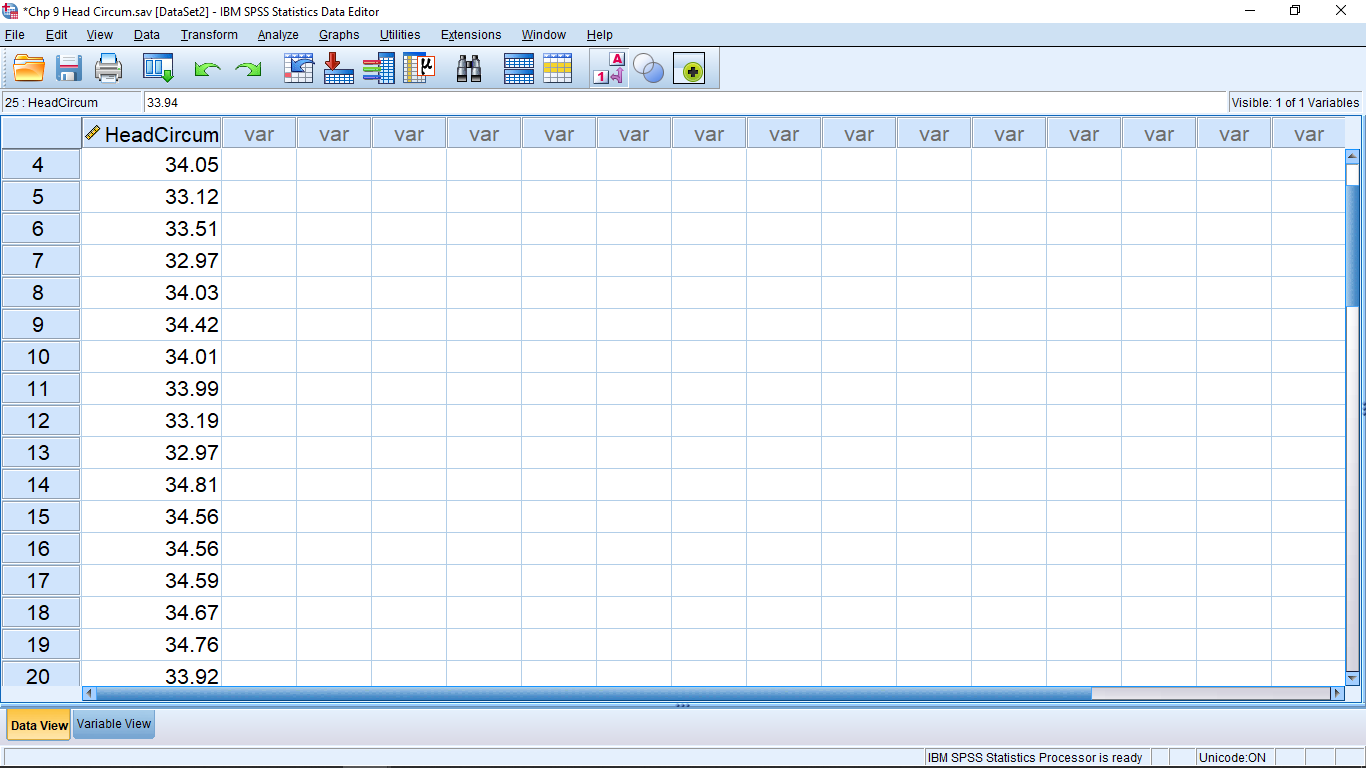
SPSS screenshot © International Business Machines Corporation.

Look at how simple it is! One variable. This is our single sample. Let’s do a $t$ -test for the hypotheses:

$H_{0}: \mu = 33.8$

(9.2) $\begin{equation*} H_{1}: \mu \neq 33.8\ \end{equation*}$

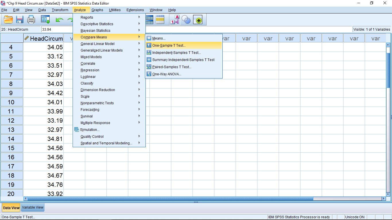
where we have used $k = 34.5$ as the potentially inferred population value. Selecting the value for $k$ is something that you will need to think about when doing single sample $t$ -tests. Some possibilities are: past values, data range midpoints or chance level values. To run the $t$ -test in SPSS, pick Analyze $\rightarrow$ Compare Means $\rightarrow$ One-Sample T Test:

The pop up menu is:

where we have moved our variable into the Test Variable(s) box. If more than one variable is in this box then a separate $t$ -test will be run for each variable. The value $k=33.8$ has been entered into the Test Value box. That’s how SPSS knows that the hypotheses to test is that of the statement (9.2) above. If you open the Options menus, you will have a chance to specify the associated confidence interval. Running the analysis gives the very simple output:

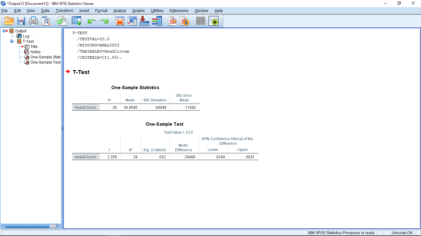
The output is simple but it requires your knowledge of the $t$ -test to interpret. As you get more experience with using SPSS, or any canned statistical software, you will get into the habit of looking for the $p$ -value. In SPSS it is in the Sig. (for Significance) column. Here $p = 0.032$ , which is less than $\alpha = 0.05$ , so we reject the null hypothesis and conclude that there is evidence that the population mean is not 34.5. Note that this $p$ -value is for a two-tailed test. What if you wanted to do a one-tailed test? Well, then you have to think because SPSS won’t do that for you explicitly. For a one-tailed test, $p = 0.016$ , half that of the two-tailed test. Remember that the two-tailed $p$ has two tails, each with an area of 0.016 as defined by $\pm t_{\rm test}$ , so getting rid of one of those areas gives the $p$ for the one- tailed test. Another way to remember to divide the two-tailed $p$ by 2 to get the one-tailed value is to remember that people try to go for a one-tailed test when they can because it has more power — it is easier to reject the null hypothesis with a one-tailed test meaning the $p$ -value will be smaller for a one-tailed test.

Let’s look at the rest of the output. There is a lot of redundant information there. You can use that redundant information to check to make sure you know what SPSS is doing and I can use that redundant information to see if you understand what SPSS is doing by reducing the redundancy and asking you to calculate the missing pieces. In the first output table, “One-Sample Statistics” is the information that you would get out of your calculator. The first three columns are $n$ , $\overline{x}$ and $s$ . The last column is $s/\sqrt{n}$ .

In the second output table “One-Sample Test”, notice that the test value of 33.8 is printed to remind you what the hypotheses being tested is. Te columns give: $t_{\rm test}$ , $\nu$ , $p$ and $\overline{x} - k$ . Notice that the first column, $t_{\rm test}$ is the fourth column $\overline{x} - k$ divided by the last column of the first table, $s/\sqrt{n}$ . The last two columns give the 95% confidence interval

(9.3) $\begin{equation*} 0.0249 < \mu - 33.80 < 0.5031 \end{equation*}$

Note that zero is not in this confidence interval which is consistent with rejecting the null hypothesis. Simply add $k=33.80$ to Equation (9.3) to get the form we go for when we do confidence intervals by hand:

(9.4) $\begin{equation*} 33.8249 < \mu < 34.3031 \end{equation*}$

You can use the output here to compute a further quantity, known as standardized effect size. You’ll get a little practice with doing that in the assignments. The standardized effect size, $d$ , is a purely descriptive statistic (although it can be used in power calculations) and is defined by

(9.5) $\begin{equation*} d = \frac{\overline{x}-k}{s} = \frac{t}{\sqrt{n}} \end{equation*}$

where, by $t$ we mean $t_{\rm test}$ . Being a descriptive statistic, people use the following rule of thumb to describe $d$ . If $d$ is approximately 0.2 then $d$ is considered “small”; if $d$ is approximately 0.5 then $d$ is considered “medium”; $d$ is approximately 0.8 then $d$ is considered “large”.

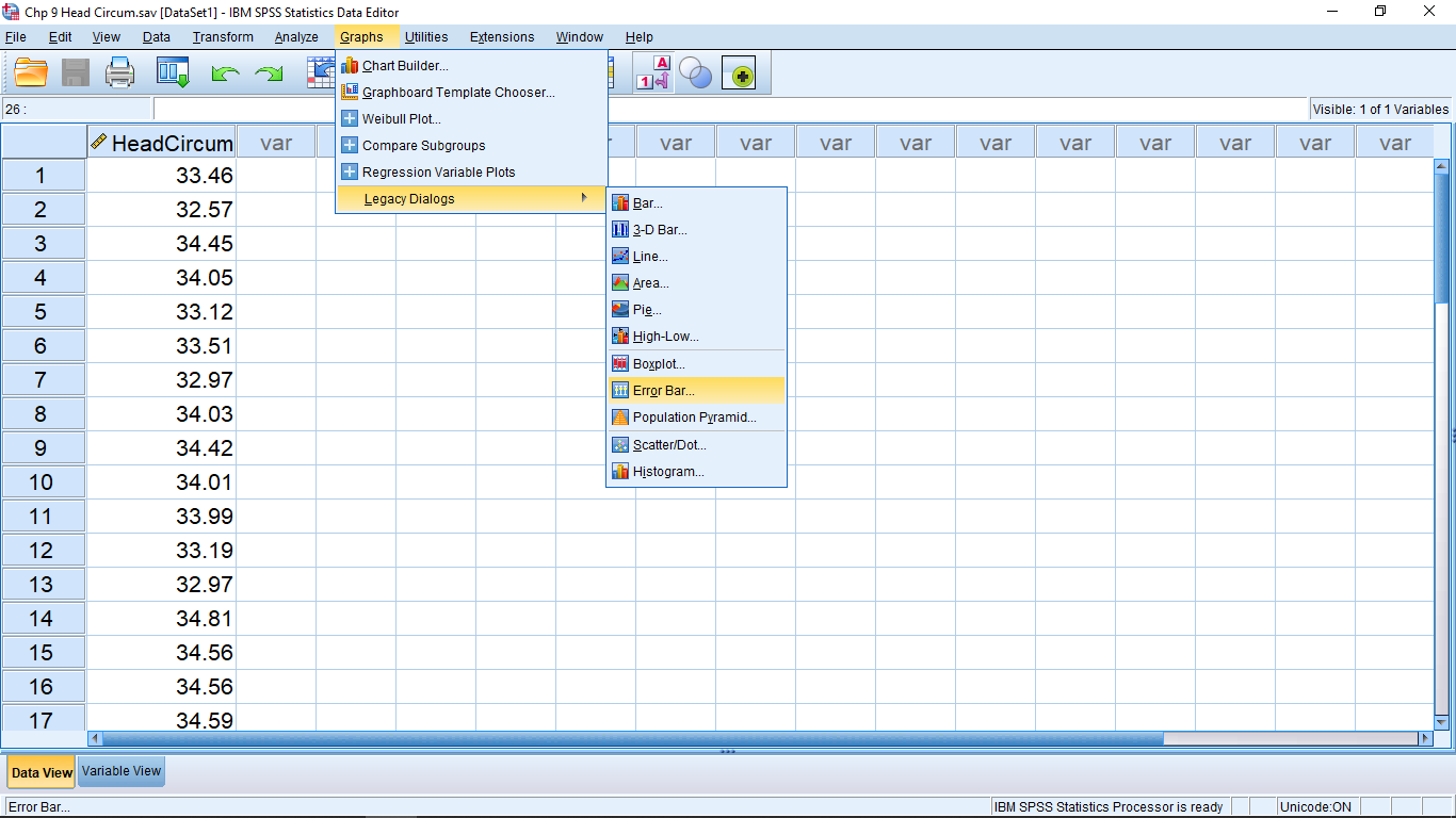
For the presentation of data graphically in reports and papers, an error bar plot is frequently used. To get such a plot for the data here, select Graphs $\rightarrow$ Legacy Dialogs $\rightarrow$ Error Bar:

Choose Simple and “Summaries of separate variables”:

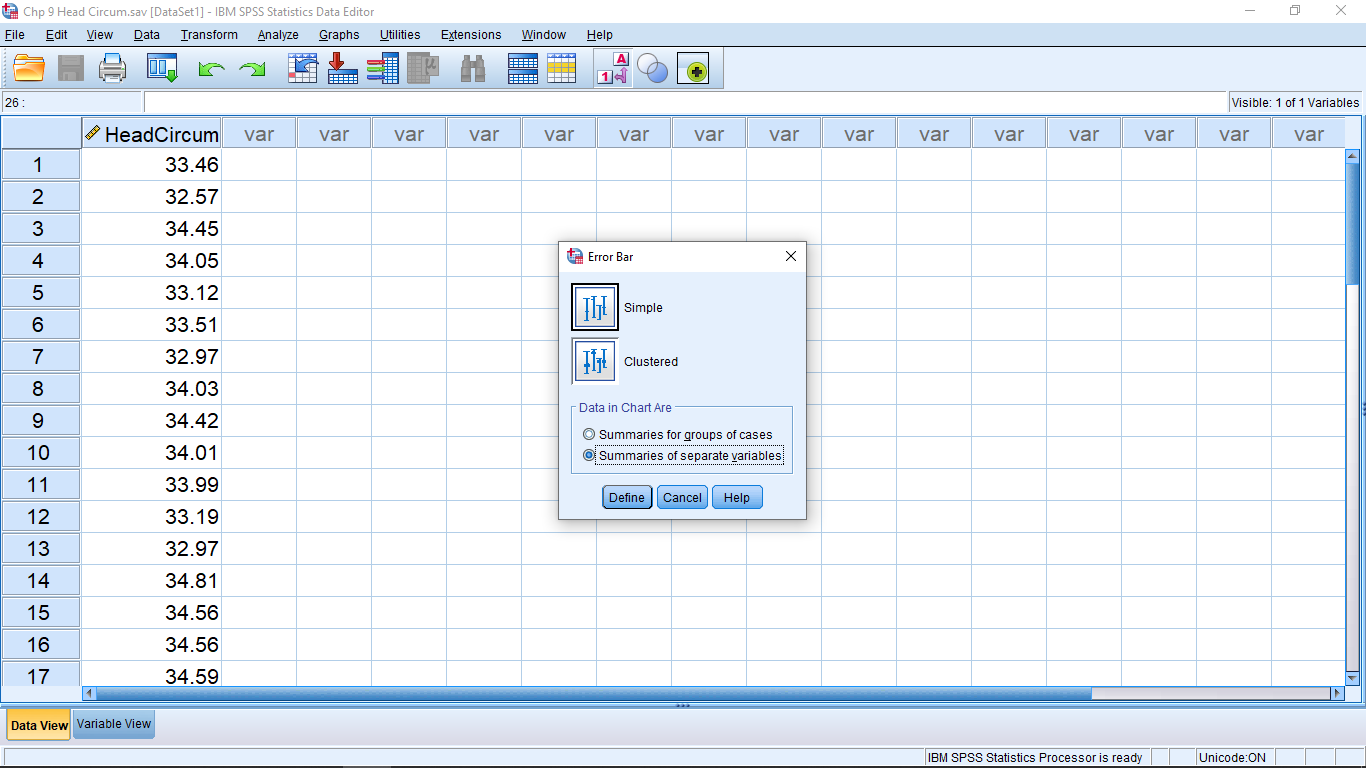
and hit Define. Then set up the menu as follows:

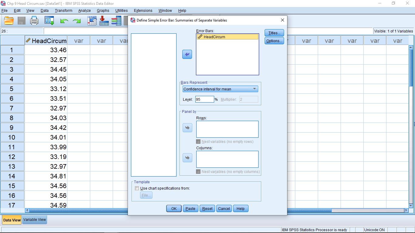
noting that we have chosen “Bars Represent” as “Standard error of the mean” so that the error bars will be $\overline{x} \pm \frac{s}{\sqrt{n}}$ :

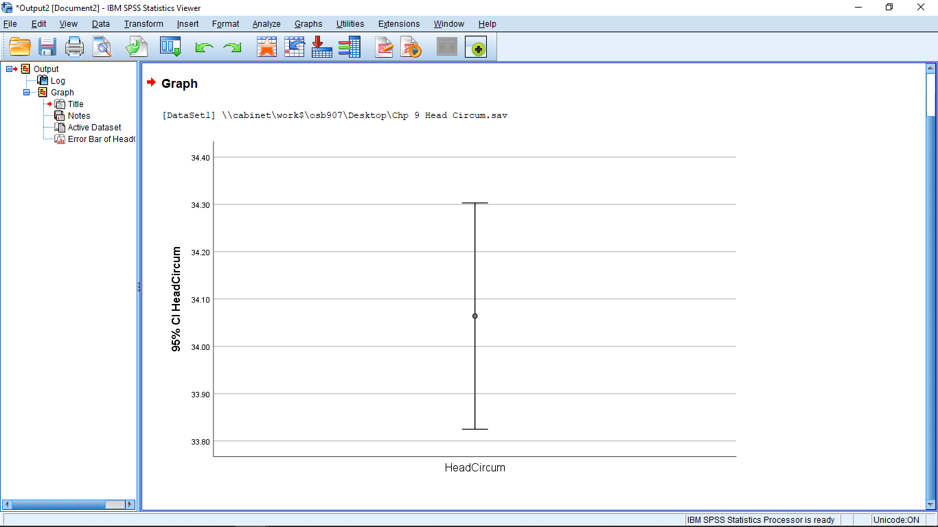
With an error bar plot like this, you can intuitively check the meaning of rejecting $H_{0}$ from the formal $t$ -test. Here the error bars do not include the value of 33.80 which is consistent with the conclusion that we reject 33.80 as a possible value for the population mean. We can see this more directly, and exactly, if we choose the value 95 $%$ confidence interval in the Bars Represent pull down of the plot menu.

This is a plot of Equation (9.4). The value $k=33.80$ is not in the 95% confidence interval.

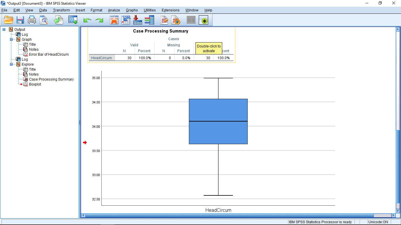
Finally, selecting Graphs $\rightarrow$ Legacy Dialogs $\rightarrow$ Boxplot gives a EDA type of data presentation:

License

Icon for the Creative Commons Attribution-NonCommercial-ShareAlike 4.0 International License

Introduction to Applied Statistics for Psychology Students Copyright © 2022 by Gordon E. Sarty is licensed under a Creative Commons Attribution-NonCommercial-ShareAlike 4.0 International License, except where otherwise noted.

License

Share This Book