5.2 **The Normal Distribution as a Limit of Binomial Distributions

Gordon E. Sarty

5. The Normal Distributions

5.2 **The Normal Distribution as a Limit of Binomial Distributions

The results of the derivation given here may be used to understand the origin of the Normal Distribution as a limit of Binomial Distributions^[1]. A mathematical “trick” using logarithmic differentiation will be used.

First, recall the definition of the Binomial Distribution^[2] as

(5.2) $\begin{equation*} w_{n}(x) = \left(\!\! \begin{array}{c} n \\ x \end{array}\!\! \right) p^{x} q^{n-x} \end{equation*}$

where $p$ is the probability of success, $q = 1 - p$ is probability of failure and

(5.3) $\begin{equation*} \left(\!\! \begin{array}{c} n \\ x \end{array}\!\! \right)= \frac{n!}{x!(n-x)!} \end{equation*}$

is the binomial coefficient that counts the number of ways to select $x$ items from $n$ items without caring about the order of selection. Here $x$ is a discrete variable, $x \in \mathbb{Z}$ , with $0 \leq x \leq n$ .

The trick is to find a way to deal with the fact that $x \in \mathbb{Z}$ ( $x$ is a discrete variable) for the Binomial Distribution and $x \in \mathbb{R}$ ( $x$ is a continuous variable) for the Normal Distribution^[3] In other words as we let $n \rightarrow \infty$ we need to come up with a way to let $\Delta x$ shrink^[4] so that a probability density limit (the Normal Distribution) is reached from a sequence of probability distributions (modified Binomial Distributions). So let $w(x)$ represent the Normal Distribution with mean $\overline{x} = np$ and variance $\sigma^{2} = npq$ . We will show how $lim_{n \rightarrow \infty} w_{n}(x) = w(x)$ where each Binomial Distribution $w_{n}(x)$ also has mean $\overline{x} = np$ and variance $\sigma^{2} = npq$ .

The heart of the trick is to notice^[5] that

(5.4) $\begin{equation*} \frac{d}{dx} \ln w(x) = \lim_{\Delta x \rightarrow 0} \frac{w(x + \Delta x) - w(x)}{w(x) \Delta x}. \end{equation*}$

This is perfectly true for the density $w(x)$ . The trick is to substitute the distribution $w_{n}(x)$ for the density $w(x)$ in the RHS of Equation (5.4) to get :

(5.5) $\begin{equation*} \frac{w_{n}(x + \Delta x) - w_{n}(x)}{w_{n}(x) \Delta x} = \frac{w_{n}(x + 1) - w_{n}(x)}{w_{n}(x)} \end{equation*}$

because $\Delta x = 1$ . The trick is to now pretend that $w_{n}(x)$ is a continuous function defined at all $x \in \mathbb{R}$ ; we just don’t know what its values should be for non-integer $x$ . With such a “continuation” of $w_{n}(x)$ we can write^[6]

(..) $\begin{align*} \frac{d}{dx} \ln w(x) & = \lim_{n \rightarrow \infty} \frac{w_{n}(x + 1) - w_{n}(x)}{w_{n}(x)} \tag{5.6}\\ & = \lim_{n \rightarrow \infty} \frac{\left(\!\! \begin{array}{c} n \\ x+1 \end{array} \!\!\right)p^{x+1}q^{n-x-1} }{\left(\!\! \begin{array}{c} n \\ x \end{array} \!\!\right) p^{x} q^{n-x} } - 1 \tag{5.7}\\ & = \lim_{n \rightarrow \infty} \frac{n-x}{x+1} \frac{p}{q} -1. \tag{5.8} \end{align*}$

Equation (5.8) has no limit; it blows up as $n \rightarrow \infty$ . We need to transform $x$ in such a way to gain control on $\Delta x$ (getting it to shrink as $n \rightarrow \infty$ ) and to get something that converges. To do that we introduce $h = \frac{1}{\sqrt{n}}$ and a new variable $u = h(x - \overline{x}) = h(x - np)$ . With this transformation of variables, the chain rule gives

(5.9) $\begin{equation*} \frac{d}{dx} \ln w(x) = \frac{du}{dx} \frac{d}{du} \ln w(u) = h \frac{d}{du} \ln w(u) \end{equation*}$

and the RHS of Equation (5.8) becomes, using $x = \frac{u}{h} + np$

(..) $\begin{align*} \frac{n-x}{x+1} \frac{p}{q} -1 & = \frac{\left( n - \frac{u}{h} - np \right)p}{\left( \frac{u}{h} + np + 1 \right)q} \tag{5.10}\\ & = \frac{\left( n(1-p) - \frac{u}{h} \right)}{\left( \frac{u}{h} + np + 1 \right) \frac{q}{p}} \tag{5.11}\\ & = \frac{\left( nq - \frac{u}{h} \right)}{\left( \frac{uq}{hp} + nq + \frac{q}{p} \right) } \tag{5.12}\\ & = \frac{\left( 1 - \frac{u}{nhq} \right)}{\left( \frac{u}{nhp} + 1 + \frac{1}{np} \right) } \tag{5.13}\\ & = \frac{\left( 1 - \frac{u}{nhq} \right)}{\left( 1 + \frac{u + h}{nhp} \right) } \tag{5.14} \end{align*}$

Using Equation (5.9), for the LHS, and Equation (5.14), for the RHS, Equation (5.8) becomes

(..) $\begin{align*} h \frac{d}{du} \ln w(u) & = \lim_{n \rightarrow \infty} \frac{1 - \frac{u}{nhq}}{1+\frac{u+h}{nhp}} - 1 \tag{5.15}\\ & = \lim_{n \rightarrow \infty} \left( 1 - \frac{u}{nhq} \right) \left[ 1 - \frac{u+h}{nhp} + \left( \frac{u+h}{nhp} \right)^{2} - \ldots \right] - 1 \tag{5.16}\\ & = \lim_{n \rightarrow \infty} -\frac{1}{np} - \frac{u}{nhq} - \frac{u}{nhp} + O\left(\frac{1}{n}\right) \tag{5.17}\\ & = \lim_{n \rightarrow \infty} -\frac{1}{np} - \frac{u}{nhpq} + O\left(\frac{1}{n}\right) \tag{5.18}\\ &= \lim_{n \rightarrow \infty} - \frac{u}{nhpq}. \tag{5.19} \end{align*}$

where $O\left(\frac{1}{n}\right)$ means terms that will go to zero as $n \rightarrow \infty$ , and we have used the relation $\frac{1}{1+x} = 1 - x + x^{2} - x^{3} + \ldots$ to get Equation (5.16}) and $p+q=1$ to go from Equation (5.17) to Equation (5.18). Dividing both sides of Equation (5.19) by $h$ leaves

(5.20) $\begin{equation*} \frac{d}{du} \ln w(u) = \lim_{n \rightarrow \infty} - \frac{u}{nh^{2}pq} = \frac{u}{pq}. \end{equation*}$

Our transformation, with its $\sqrt{n}$ , has given us the exact control we need to keep the limit from disappearing or blowing up. Integrating Equation (5.20) gives

(5.21) $\begin{equation*} w(u) = C e^{-\frac{u^{2}}{2pq}} \end{equation*}$

where $C$ is the a constant of integration. Switching back to the $x$ variable

(..) $\begin{align*} w(x) & = C e^{-\frac{(h[x-\overline{x}])^{2}}{2pq}} \tag{5.22}\\ & = C e^{-\frac{(x-\overline{x})^{2}}{2npq}} \tag{5.23}\\ & = C e^{-\frac{(x-\overline{x})^{2}}{2\sigma^{2}}}. \tag{5.24} \end{align*}$

To evaluate the constant of integration, $C$ , we impose $\int_{-\infty}^{\infty} w(x) \: dx = 1$ because we want $w(x)$ to be a probability distribution. So

(5.25) $\begin{equation*} C \int_{-\infty}^{\infty} e^{-\frac{(x-\overline{x})^{2}}{2\sigma^{2}}} \: dx = C \sqrt{2 \pi \sigma^{2}} = 1 \end{equation*}$

so

(5.26) $\begin{equation*} C = \frac{1}{ \sqrt{2 \pi \sigma^{2}}} \end{equation*}$

and

(5.27) $\begin{equation*} w(x) = \frac{1}{ \sqrt{2 \pi \sigma^{2}}} \: e^{-\frac{(x-\overline{x})^{2}}{2\sigma^{2}}} \end{equation*}$

which is the Normal Distribution that approximates Binomial Distributions with the same mean and variance as $n$ gets large.

Figure 5.1 : The transformation $u = \frac{(x - np)}{\sqrt{n}}$ effectively shrinks the $\Delta x$ of the Binomial Distribution with mean $\overline{x} = n p$ and variance $\sigma^{2} = npq$ by pulling a continuous version $w_{n}(x)$ back to the constant Normal Distribution $w(u)$ . Another way of thinking about it is that the transformation $x = \sqrt{n} u + np$ takes the fixed Normal Distribution $w(u)$ to the Normal Distribution $w(x)$ that provides a better and better approximation of $w_{n}(x)$ as $n \rightarrow \infty$ .

Figure 5.1 : The transformation $u = \frac{(x - np)}{\sqrt{n}}$ effectively shrinks the $\Delta x$ of the Binomial Distribution with mean $\overline{x} = n p$ and variance $\sigma^{2} = npq$ by pulling a continuous version $w_{n}(x)$ back to the constant Normal Distribution $w(u)$ . Another way of thinking about it is that the transformation $x = \sqrt{n} u + np$ takes the fixed Normal Distribution $w(u)$ to the Normal Distribution $w(x)$ that provides a better and better approximation of $w_{n}(x)$ as $n \rightarrow \infty$ .

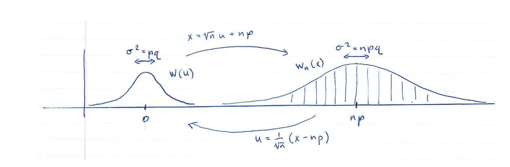
You may be wondering why that transformation $u = \frac{1}{\sqrt{n}} (x - np)$ worked because it seems to have been pulled from the air. According to Lindsay & Margenau, it was Laplace who first used this transformation and derivation in 1812. What this transformation does is pull the Binomial Distribution $w_{n}(x)$ back to have a mean of zero (by subtracting $\overline{x} = np$ ) which keeps $x$ from running off to infinity and, more importantly, allows us to define a function $w(u)$ with $u \in \mathbb{R}$ that has a constant variance of $pq$ that we can match to $npq$ when we transform back to $x$ at each $n$ , see Figure 5.1. Looking at it the other way around, the Normal Distribution^[7] $w(x)$ with $x = \sqrt{n} u + np$ is an approximation for Binomial Distribution $w_{n}(x)$ that “asymptotically” approaches $w_{n}(x)$ as $n \rightarrow \infty$ .

This is not the only way to form a probability density limit from a sequence of Binomial distributions. It is one that gives a good approximation of the Binomial Distribution when $n$ is fairly small if the term $\frac{1}{np}$ in Equation (5.18) becomes small quickly. If $p$ is very small, this does not happen and another limit of Binomial Distributions that leads to the Poisson Distribution is more appropriate. When $p$ and $q$ are close to 0.5 or more generally when $np \geq 5$ and $nq \geq 5$ then the Normal approximation is a good one. Either way, the density limit is a mathematical idealization, a convenience really, that is based on a discrete probability distribution that just summarizes the result of counting outcomes. Counting gives the foundation for probability theory.

The formula for the Binomial Distribution was apparently derived by Newton according to: Lindsay RB, Margenau. Foundations of Physics. Dover, New York, 1957 (originally published 1936). For that claim, Lindsay & Margenau quote: von Mises R. Probability, Statistics, and Truth. Macmillan, New York, 1939 (originally published 1928). The derivation of the Normal Distribution presented here largely follows that given in Lindsay & Margenau's book. ↵
In class we denoted the Binomial distribution as $P(x \mid n)$ . Here we use $w_{n}(x) = P(x \mid n)$ to avoid using too many P's and p's. ↵
Remember that the Normal Distribution is technically a probability density but we slur the use of the word distribution between probability distribution (discrete $x$ ) and probability density (continuous $x$ ) like everyone else. ↵
$\Delta x = 1$ for the Binomial Distribution. ↵
Remember that $\frac{d}{dx} \ln(x) = \frac{1}{x}$ and use the chain rule to notice this. ↵
You can probably imagine many ways to continue the Binomial Distribution from $x \in \mathbb{Z}$ to $x \in \mathbb{R}$ . It doesn't matter which one you pick as long as the behaviour of your new function is not too crazy between the integers; that is, $\lim_{n \rightarrow \infty} w_{n}(x)$ should exist at all $x \in \mathbb{R}$ . ↵
Our symbols here are not mathematically clean; we should write something like $w(u(x))$ instead of $w(x)$ or $w$ composed with $u$ at $x$ , $w \circ u_{n}(x)$ , instead of $w(x)$ . But to emphasize the intuition we use $w(x)$ . In clean symbols, the function $w \circ u_{n}(x)$ asymptotically approaches $w_{n}(x)$ where $u_{n}(x) = \frac{(x - np)}{\sqrt{n}}$ . ↵