3.4 SPSS Lesson 2: Combining variables and recoding

Frequently data collection results in a collection of many variables. This happens, for example, with tests or surveys where people answer questions on a 5 or 7 point Lickert scale where questions range from, say, “strongly agree” to “somewhat agree” to to “strongly disagree”. A bunch of those questions may refer to, say, happiness and adding up the scores, perhaps averaging them, will lead to a single variable, one dependent variable, that becomes our measurement of happiness. This gives us not only a univariate variable that we can subject to a statistical test but likely gives us a stronger and more reliable measurement of happiness. A problem with combining variables in this way arises if the response “1” for “strongly agree” means happiness for one question (e.g. “I wake up happy”) and sadness in another question (e.g. “I go to bed sad”). In such a situation some of the variables will need to be reverse-scaled or recoded before they can be added. Let’s see how to combine and recode variables in SPSS.

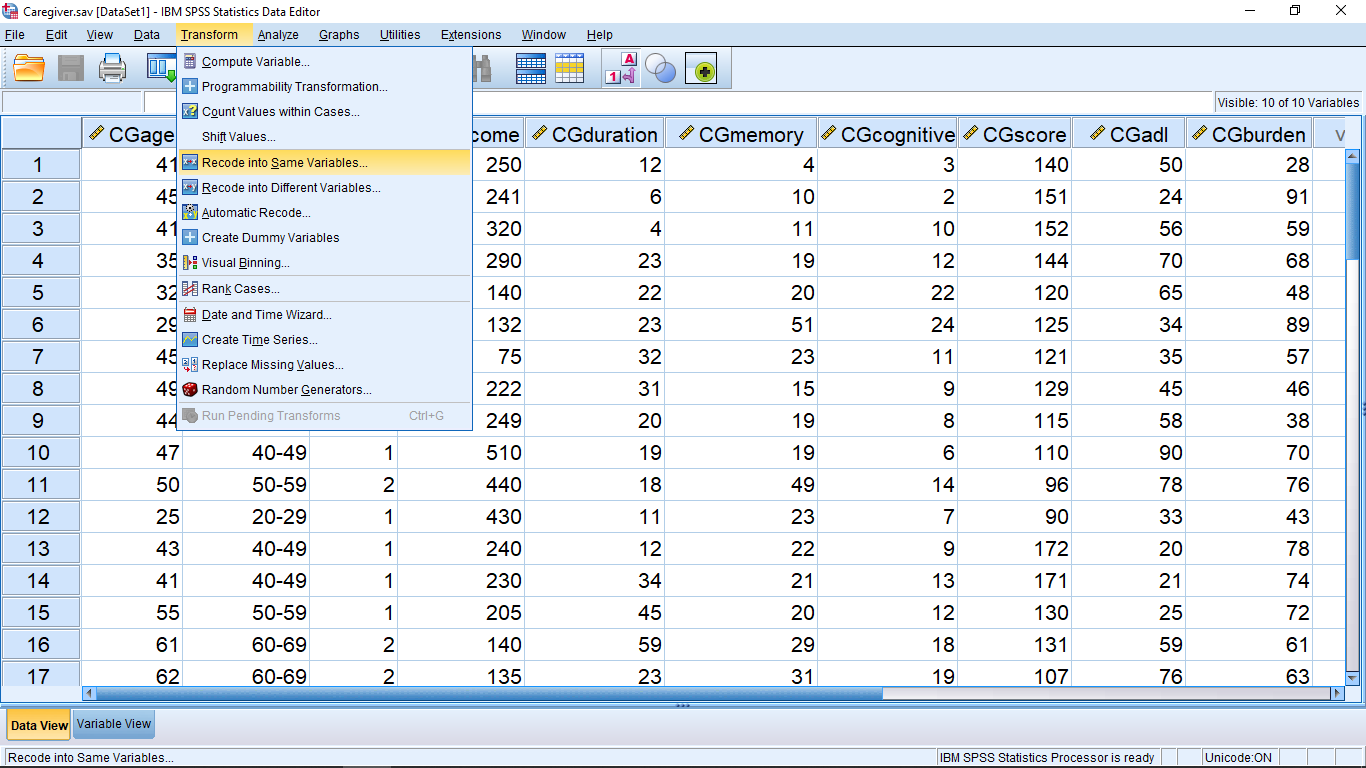
Open the file “Caregiver.sav” from the textbook Data Sets. This dataset is about the different attributes of diamonds such as its color, price, carat, cutting quality etc. Here one of the variables is cut\_new which basically represents the cutting quality of diamond and takes values from 1 to 5 depending on the cutting quality with 5 being the best quality. Now let’s assume that we need to reverse scale this variable to use it in other calculations in a meaningful manner. To recode cut\_new first open the Transform Recode in Same Variables… menu :

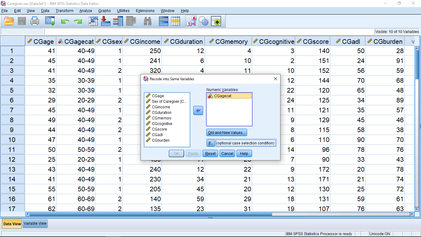
You can choose the Recode into Different Variables… if you want to, instead. That choice will lead to the creation of a new variable that you would use in place of cut\_new for your analysis. With our choice of Recode in Same Variables… we will overwrite the old values of cut\_new with new ones. (This is a danger if you make a mistake.) Our job is now to map 1 to 5, 2 to 4, 3 to 3, 4 to 2 and 5 to 1, recoding the variable. First move the cut\_new variable over in the pop up menu :

then hit the Old and New Values.. button that will bring up a new pop up menu. Next enter 1 under Old Value and 5 in New Value :

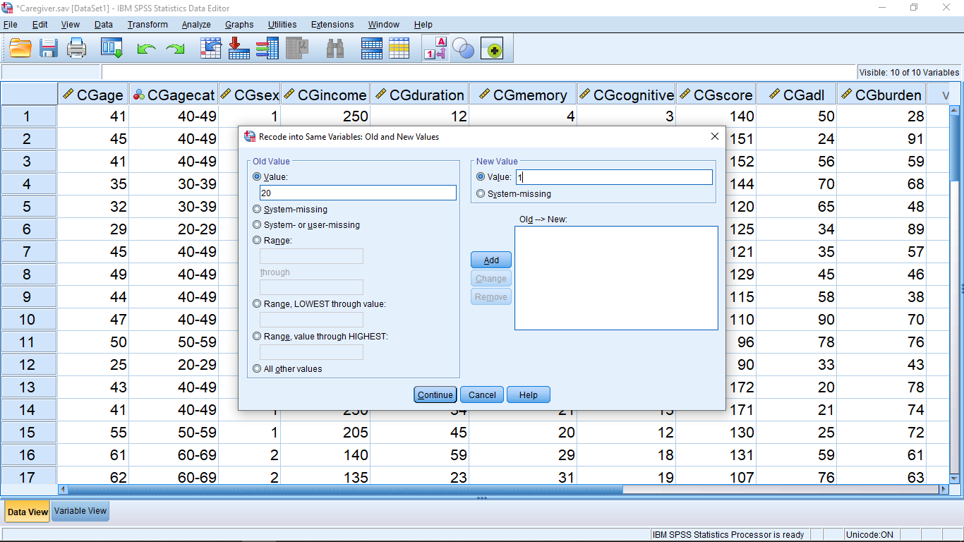
then hit Add :

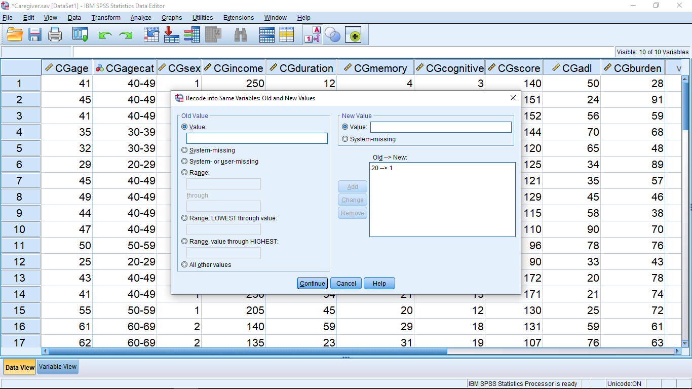
Continue this way to complete the recoding list :

Hit Continue, then OK. The variable cut\_new will now have the new values in the Data View window.

Now suppose we want to add multiple variables to create a new variable. Let’s open the dataset Caregiver from the course website. This dataset is regarding the test scores of students from diverse background in UK. Here we will add the test scores of read, write, math and science to create a new variable totalscore. Pick the Transform Compute Variable… menu :

This will bring up a menu which is essentially the calculator feature of SPSS :

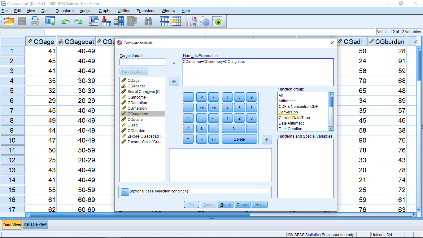
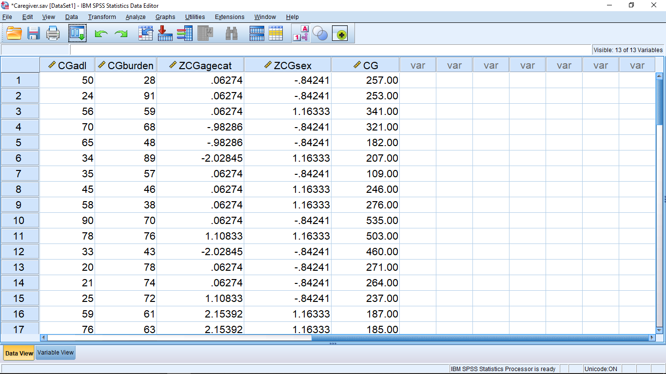
Fill in the menu as shown above. You can move variable names into the Numeric Expression box by double clicking on the variable name, by clicking on the variable name and the arrow or by simply typing it. There are fancier ways to get a sum of variables experesion in Numeric Expression, but we will keep it simple for now. The target variable name is totalscore which, after you hit OK, shows up as a new variable, ready for statistical analysis, in the last column in the Data View window :

Let’s do a couple of (descriptive) analysis with this new variable. Let’s take Caregiver as our dataset. Suppose we want to find the median of the totalscore values. To do this task by hand, we need to put the data in order from smallest to largest. This is tedious but SPSS can do it with a couple of mouse clicks (yes, yes SPSS can compute the median directly but whatever). There are a couple of approaches in SPSS to ordering, or ranking, data. One is to compute the rank, that is, give rank 1 to the lowest value, 2 to the next lowest up to for the highest value. Pick Transform Rank Cases and move totalscore into the Variable(s) box :

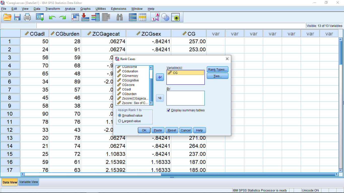
This is a new menu for us, so let’s take a look at the submenus. First, the Rank Types menu :

Pretty fancy. Much to advanced for our use, so let’s leave that one be, hit Continue. Next look at Ties…

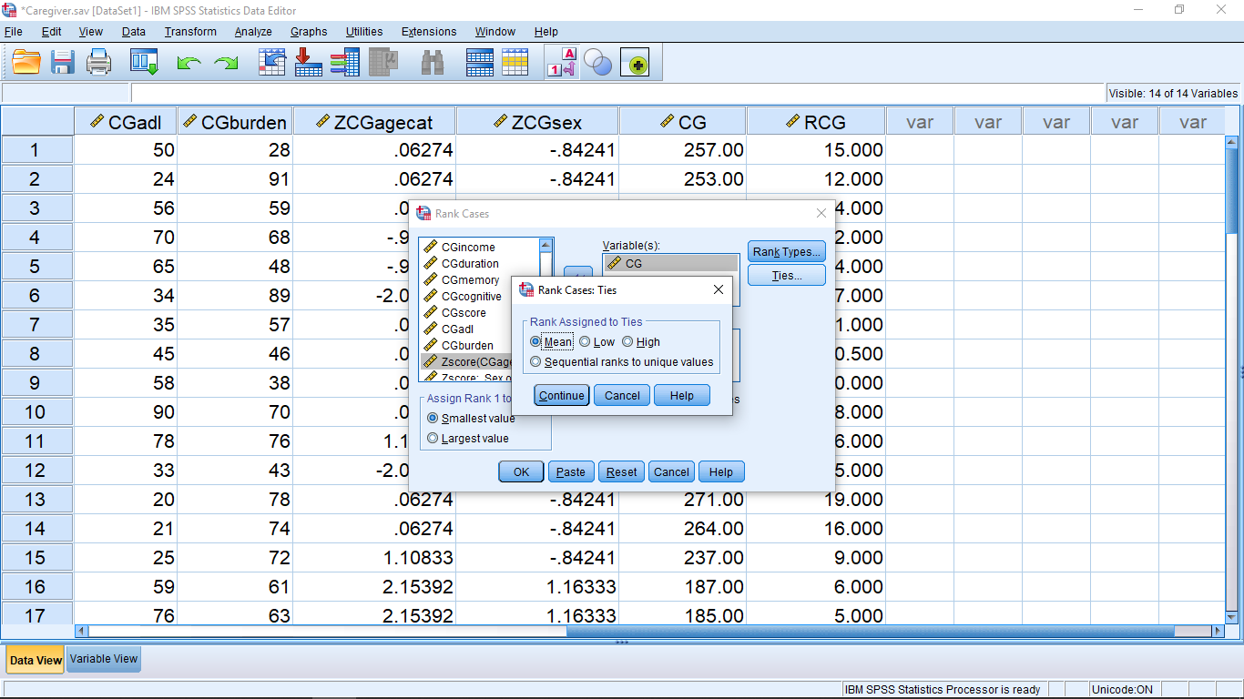
We will assign the average (mean) rank to ties in out classes. To understand the ties options, think of two people in a race who cross the finish line at exactly the same time, a tie. With the mean rank, they both come in 1.5 place. With lowest, they both come in 1st place, with highest, they both come in 2nd place. Hit Continue, the OK and a new variable Rtotalscore with be formed in the Data View menu :

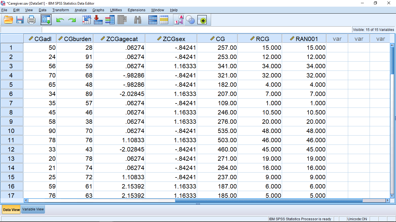
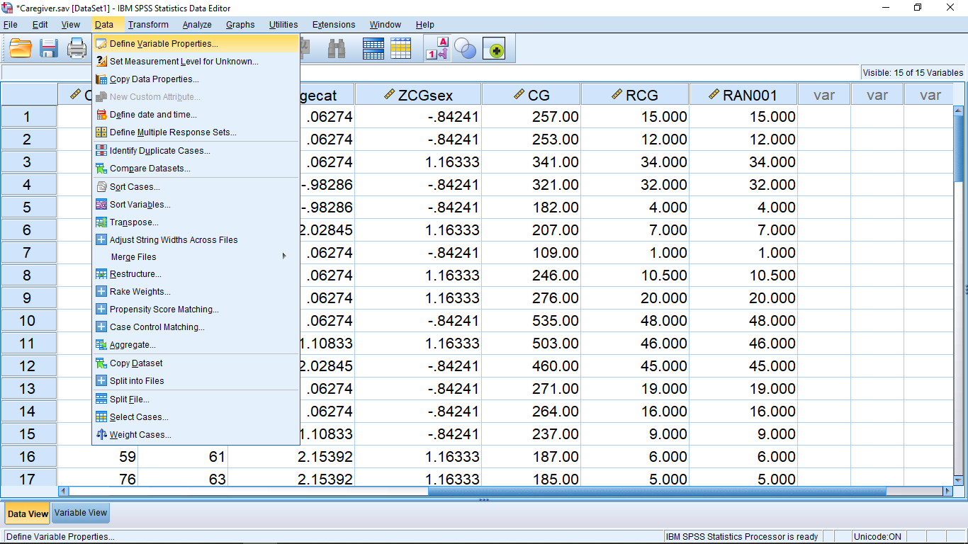
Here the variable RCG ranks the total score of the students. But it’s very difficult from this data view to identify which students’ rank the highest or lowest, let alone who falls in the middle to find the median. This is not quite what we are after to easily get the median. Ranking will become useful on Psy 234 (in Chapter 16), but it’s not that useful for us now. What we need, is to shuffle the numbers around from lowest to highest (of course we can do that directly). To shuffle pick Data Sort Cases :

which brings up, after moving over the RCG total score variable :

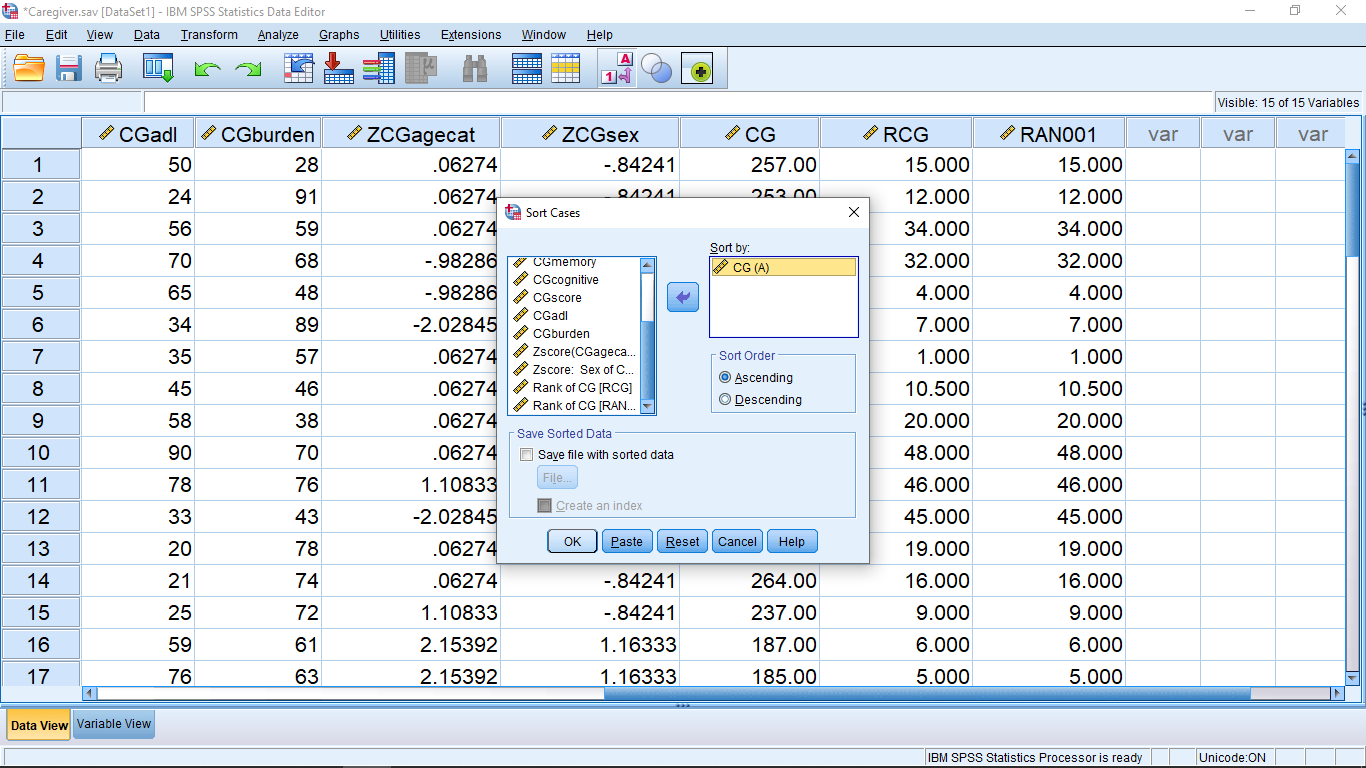
Keep the ascending button selected (sort from lowest to highest), then hit OK to sort the file :

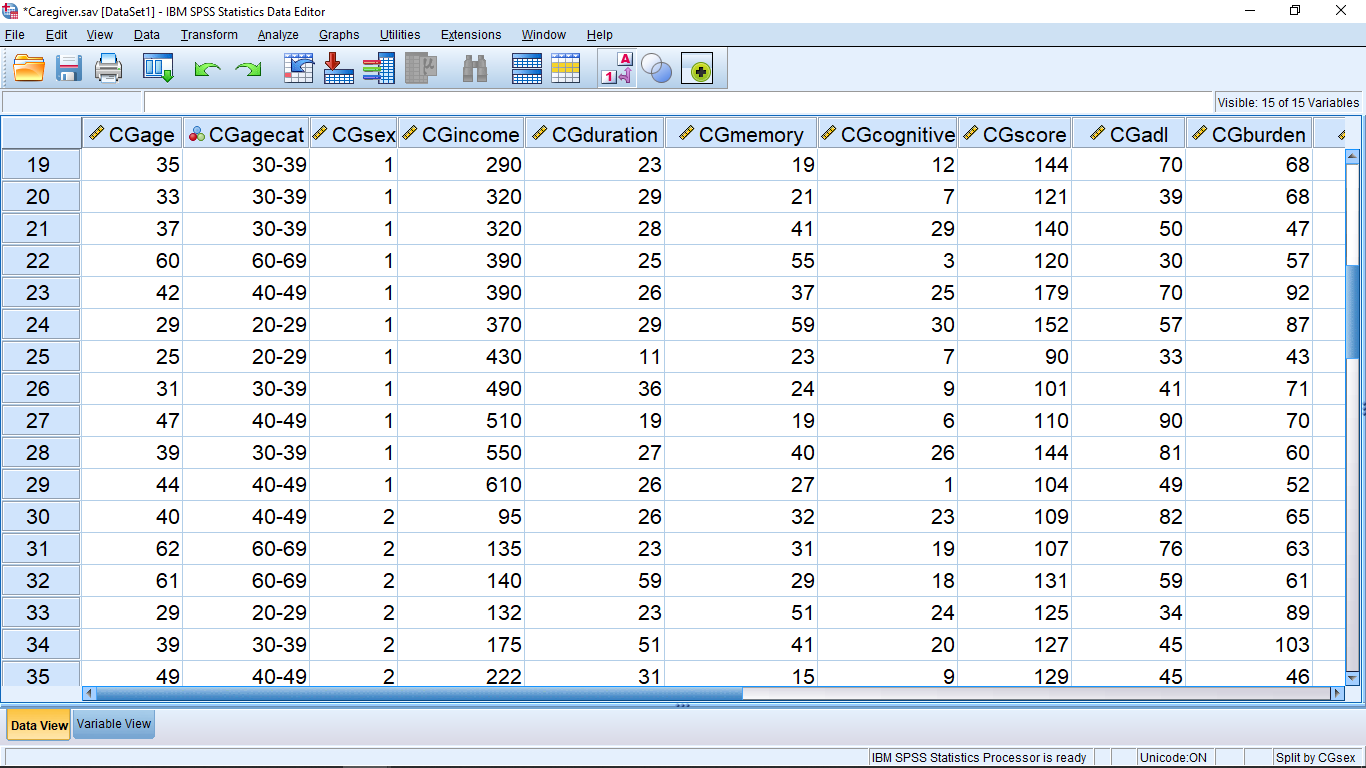
Everything is sorted now. (Note how useful the id variable is now. If that wasn’t there, we’d lose track of who’s data was what.) Now if we scroll down, we will find that the middle two total test scores are both 210. Thus the median of total score is 210.

As a final analysis of the Caregiver data, suppose we wanted some descriptive statistics for the male students separate from the female students. To do this we use the “split file” feature of SPSS. Select Data Split File to get

where the gender variable has been moved into the “Groups Based on” box — you will need to click on the “Organize output by groups” button also. We’ll also leave the “Sort the file by grouping variables” (gender in this case), this will shuffle the file yet again, putting all the males and females together. So, when you hit OK the result is

Now the file is sorted into Male and Female (the 1-A button at the top has been pressed). Also note that “Split by gender” appears on the lower right corner of the Data View window. Now let’s do a simple descriptive statistics analysis of the total score variable. The output looks like :

To unsplit the file, go back to Data Split File and hit the “Analyze all cases, do not create groups” button. This will remove the “Split” message from the lower right corner and when the descriptive statistics is run again, you will get :

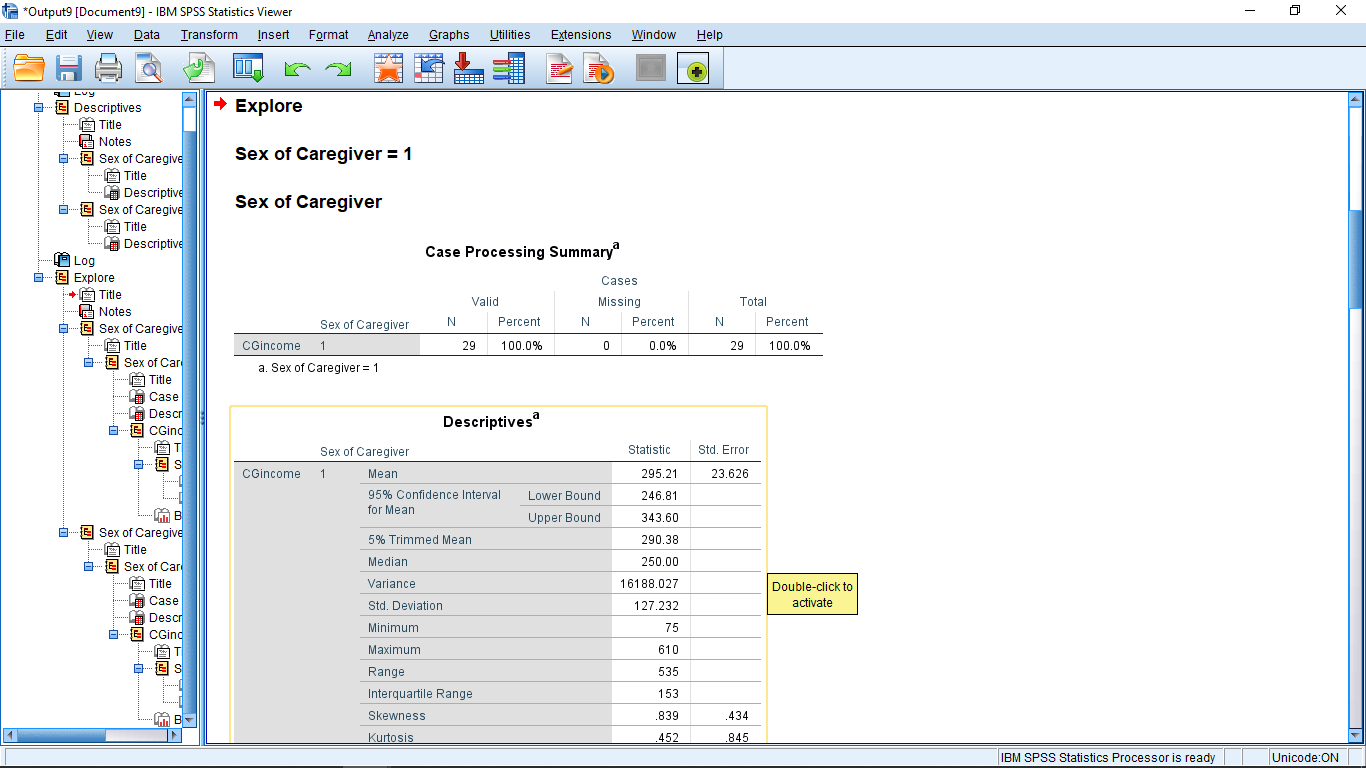
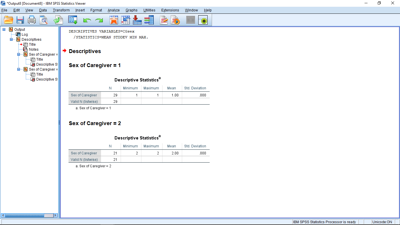
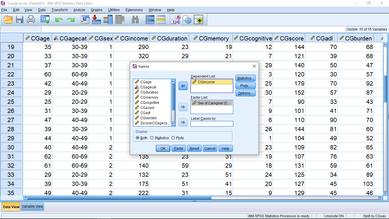
From here, with the file unsplit, we can use gender as a factor to get separate descriptive statistics for males and female. Select Analyze Explore and use gender as the factor, which results in :

From here, with the file unsplit, we can use gender as a factor to get separate descriptive statistics for males and female. Select Analyze Explore and use gender as the factor :

The result is :