8.1 Confidence Intervals Using the z-Distribution

Gordon E. Sarty

8. Confidence Intervals

8.1 Confidence Intervals Using the z-Distribution

With confidence intervals we will make our first statistical inference. Confidence intervals give us a direct inference about the population from a sample. The probability statement is one about hypotheses about the mean $\mu$ of the population based on the mean $\overline{x}$ and standard deviation $s$ of the sample. This is a fine point. The frequentist definition of probability gives no way to assign a probability to a hypothesis. How do you count hypotheses? The central limit theorem makes a statement about the sample means $\overline{x}$ on the basis of a hypothesis about a population, about its mean $\mu$ and standard deviation $\sigma$ . If the population is fixed then the central limit theorem gives the results of counting sample means, frequentist probabilities. If we let $H$ represent a hypothesis about a population (i.e. that it is described by $\mu$ and $\sigma$ ) and let $D$ represent data (with mean $\overline{x}$ ) then the central limit theorem gives the probability $P(D \mid H) = P(\overline{x} \mid \mu, \sigma)$ . The confidence intervals that we’ll look at first give $P(H \mid D) = P(\mu \mid \overline{x}, \sigma)$ . We’ll look at the recipe for computing confidence intervals for means first, then return to this discussion about probabilities for hypotheses.

Our goal is to define a symmetric interval about the population mean $\mu$ that will contain all potentially measured values of $\bar{x}$ with a probability^[1] of $\cal{C}$ .

Typically $\cal{C}$ will be

${\cal{C}} = 0.90 \hspace{.5in} \mbox{(90\% confidence)}$

${\cal{C}} = 0.95 \hspace{.5in} \mbox{(95\% confidence)}$

${\cal{C}} = 0.99 \hspace{.5in} \mbox{(99\% confidence)}$

The assumptions that we need in order to use the $z$ -distribution to compute confidence intervals for means are :

The population standard deviation, $\sigma$ , is known (a somewhat artificial assumption since it is usually not known in an experimental situation) or
The sample size is greater than (or equal to) 30, $n \geq 30$ and we use $\sigma = s$ , the sample standard deviation in our confidence interval formula.

Definition : Let $z_{\cal{C}} = z_{\alpha/2}$ where ${\cal{C}} = 1 - \alpha$ be the $z$ -value, from the Standard Normal Distribution Table that corresponds to an area, between 0 and $z_{\cal{C}}$ of ${\cal{C}}/2$ as shown in Figure 8.1.

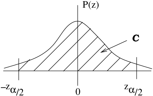Figure 8.1 : The $z$ -distribution areas of interest associated with $z_{\cal{C}} = z_{\alpha/2}$ .

To get our confidence interval we simply inverse $z$ -transform the picture of Figure 8.1, taking the mean of 0 to the sample mean $\bar{x}$ and the standard deviation of 1 to the standard error $\sigma/\sqrt{n}$ as shown in Figure 8.2.

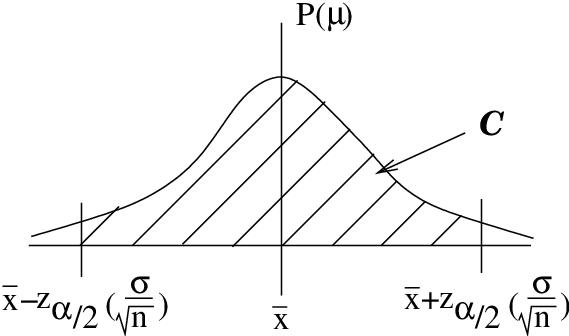Figure 8.2 : The inverse $z$ -transformation of Figure 8.1 gives the confidence interval for $\mu$ .

So here is our recipe from Figure 8.2. The $\cal{C}$ -confidence interval for the mean, under one of the two assumptions given above, is :

$\bar{x} - z_{\alpha/2} \left( \frac{\sigma}{\sqrt{n}}\right) < \mu < \bar{x} + z_{\alpha/2} \left( \frac{\sigma}{\sqrt{n}}\right)$

or using notation that we will use as a standard way of denoting symmetric confidence intervals

(8.1) $\begin{equation*} \bar{x} - E < \mu < \bar{x} + E \end{equation*}$

where

$E = z_{\cal{C}} \left( \frac{\sigma}{\sqrt{n}}\right).$

The notation $z_{\cal{C}}$ is more convenient for us than $z_{\alpha/2}$ because we will use the t Distribution Table in the Appendix to find $z_{\cal{C}}$ very quickly. We could equally well write

$\mu = \bar{x} \pm E$

but we will use Equation (8.1) because it explicitly gives the bounds for the confidence interval.

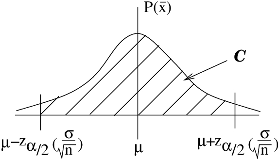
Notice how the confidence interval is backwards from the picture that the central limit theorem gives, the picture shown in Figure 8.3. We actually had no business using the inverse $z$ -transformation $\mu = (z - \bar{x})/(\sigma/\sqrt{n})$ to arrive at Figure 8.2. It reverses the roles of $\mu$ and $\bar{x}$ . We’ll return to this point after we work through the mechanics of an example.

Figure 8.3 : The central limit theorem is about distributions of sample means.

Example 8.2 : What is the 95 $\%$ confidence interval for student age if the population $\sigma$ is 2 years, sample $n = 50$ , $\bar{x} = 23.2$ ?

Solution : So ${\cal{C}} = 0.95$ . First write down the formula prescription so you can see with numbers you need:

$\bar{x} - E < \mu < \bar{x} + E \mbox{\hspace{2em}where\hspace{2em}} E = z_{95\%} \frac{\sigma}{\sqrt{n}}.$

First determine $z_{\cal{C}} = z_{\alpha/2}$ . With the tables in the Appendices, there are two ways to do this. The first way is to use the Standard Normal Distribution Table noting that we need the $z$ associated with a table area of $0.95/2 = 0.475$ . Using the table backwards we find $z_{\cal{C}} = 1.96$ . The second way, the recommended way especially during exams, is to use the t Distribution Table. Simply find the column for the 95 $\%$ confidence level and read the $z$ from the last line of the table. We quickly find $z_{95\%} = 1.960$ .

Either way we now find

$E = 1.96( \frac{2}{\sqrt{50}}) = 0.6$

so

$\begin{eqnarray*} \bar{x} - E &< \mu <& \bar{x} + E\\ 23.2 - 0.6 &< \mu <& 23.2 + 0.6 \\ 22.6 &< \mu <& 23.8 \end{eqnarray*}$

with 95 $\%$ confidence.

▢

Because of this issue about probabilities of hypotheses, many prefer to say "confidence" and not probability. But we will learn enough about Bayesian probability to say "probability". ↵

License

Icon for the Creative Commons Attribution-NonCommercial-ShareAlike 4.0 International License

Introduction to Applied Statistics for Psychology Students Copyright © 2022 by Gordon E. Sarty is licensed under a Creative Commons Attribution-NonCommercial-ShareAlike 4.0 International License, except where otherwise noted.

License

Share This Book