12.1 One-way ANOVA

Gordon E. Sarty

12. ANOVA

12.1 One-way ANOVA

A one-way ANOVA (ANalysis Of VAriance) is a generalization of the independent samples $t$ -test to compare more than 2 groups. (Actually an independent samples $t$ -test and an ANOVA with two groups are the same thing). The hypotheses to be tested, in comparing the mean of $k$ groups, with a one-way ANOVA are :

$\begin{eqnarray*} & H_{0}: & \mu_{1} = \mu_{2} = \ldots = \mu_{k} \\ & H_{1}: & \mbox{ At least one of the means is different from the others.} \end{eqnarray*}$

The following assumptions must be met for ANOVA (the version we have here) to be valid :

Normally distributed populations (although ANOVA is robust to violations of this condition).
Independent samples (between subjects).
Homoscedasticity : $\sigma_{1}^{2} = \sigma_{2}^{2} = \ldots = \sigma_{k}^{2}.$ (ANOVA is robust to violations of this too, especially for larger sample sizes.)

The concept of ANOVA is simple but we need to learn some terminology so we can understand how other people talk about ANOVA. Each sample set from each population is referred to as a group or each population is called a group.

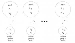
There will be $k$ groups with sample sizes $n_{1}$ , $n_{2}$ , $\ldots$ , $n_{k}$ with the total number of data points being $N = \sum_{i=1}^{k} n_{i}$ . For an ANOVA, the concept of independent variable (IV) and dependent variable (DV) become important (the IV in a single sample or a paired $t$ -test is trivially a number like $k$ or 0). The groups comprise different values of one IV. The IV is discrete with $k$ values or levels.

In raw form, the test statistic for a one-way ANOVA is

$F_{\rm test} = F_{\nu_{1},\nu_{2}} = \frac{s_{\rm B}^{2}}{s_{\rm W}^{2}}$

where

$\nu_{1} = k-1 \mbox{ (d.f.N.) \ \ \ } \nu_{2} = N-k \mbox{ (d.f.D.) \ \ \ }$

are the degrees of freedom you use when looking up $F_{\rm crit}$ in the F Distribution Table and where

$s_{\rm B}^{2} = \frac{\sum_{i=1}^{k} n_{i} (\bar{x}_{i}- \bar{x}_{\rm GM})^{2}}{k-1}$

is the variance between groups, and

$s_{\rm W}^{2} = \frac{\sum_{i=1}^{k}(n_{i}-1) s_{i}^{2}}{\sum_{i=1}^{k}(n_{i}-1)}$

is the variance within groups. Here $n_{i}$ , $\bar{x}_{i}$ and $s_{i}$ are the sample size, mean and standard deviation for sample $i$ and $\bar{x}_{\rm GM}$ is the grand mean:

$\overline{x}_{\rm GM} = \frac{\sum_{i=1}^{k}\sum_{j=1}^{n_{i}} x_{ij}}{N} = \frac{\sum_{i=1}^{k} n_{i}\overline{x}_{i}}{N}$

where $x_{ij}$ is data point $j$ in group $i$ .

So you can see that ANOVA, the analysis of variance, is about comparing two variances. The within variance $s_{\rm W}^{2}$ is the variance of all the data lumped together, just as the grand mean $\bar{x}_{\rm GM}$ is the mean of all the data lumped together. It is the noise. You can see that the within variance is the weighted mean (weighted by $n_{i}-1$ ) of the group sample variances — a little algebra shows that this is the variance of all the data lumped together. The between variance $s_{\rm B}^{2}$ a variance of the sample means $\bar{x}_{i}$ . It is the signal. If the sample means were all exactly the same then the between variance $s_{\rm B}^{2}$ would be zero. So the higher $F_{\rm test}$ the more likely the means are different. $F_{\rm test}$ is a signal-to-noise ratio. If the means were all the same in the population then $s_{\rm B}^{2}$ would follow a $\chi_{k-1}^{2}$ distribution and $s_{\rm W}^{2}$ (whether the population means were the same or not) would follow a $\chi_{N-k}^{2}$ distribution. Thus if the population means were all the same ( $H_{0}$ ) then the $F$ test statistic follows a $F_{\nu_{1},\nu_{2}}$ distribution which has an expected value^[1] (mean) of about 1. $F_{\rm test}$ must be sufficiently bigger than 1 to reject $H_{0}$ .

The analysis of the variances can be broken down further, to sums of squares, with the following definitions^[2] :

$\begin{eqnarray*}s_{\rm B}^{2} = {\rm MS}_{\rm B} \mbox{\ \ \ \ between groups mean square}\end{eqnarray*}$

and

$\begin{eqnarray*}s_{\rm W}^{2} = {\rm MS}_{\rm W} \mbox{\ \ \ \ within groups mean square.}\end{eqnarray*}$

Next we note that $\nu_{1} = k-1$ and $\nu_{2} = N - k = \sum_{i=1}^{k} (n_{i} - 1)$ so

$\begin{eqnarray*}{\rm MS}_{\rm B} = \frac{{\rm SS}_{\rm B}}{\nu_{1}}\end{eqnarray*}$

and

$\begin{eqnarray*}{\rm MS}_{\rm W} = \frac{{\rm SS}_{\rm W}}{\nu_{2}}\end{eqnarray*}$

where

$\begin{eqnarray*}{\rm SS}_{\rm B} = \sum_{i=1}^{k} n_{i} (\bar{x}_{i} - \bar{x}_{\rm GM})^{2} \mbox{\ \ \ sum of squares between groups} \label{ssb}\end{eqnarray*}$

and

$\begin{eqnarray*}{\rm SS}_{\rm W} = \sum_{i=1}^{k} (n_{i}-1) s_{i}^{2} \mbox{\ \ \ sum of squares within groups}\end{eqnarray*}$

so that

$\begin{eqnarray*}F_{\rm test} = \frac{{\rm MS}_{\rm B}}{{\rm MS}_{\rm W}}\end{eqnarray*}$

Why are sums of squares so prominent in statistics? (They will show up in linear regression too.) Because squares are the essence of variance. Look at the formula for the normal distribution, Equation 5.1. The exponent is a square. Mean and variance are all you need to completely characterize a normal distribution. Means are easy to understand, so sums of square focus our attention to the variance of normal distributions. If we make an assumption that all random noise has a normal distribution (which can be justified on general principles) then the sums of squares will tell the whole statistical story. Sums of squares also tightly links statistics to linear algebra (see Chapter 17) because the Pythagorus Theorem, which gives distances in ordinary geometrical spaces, is about sums of squares.

Computer programs, like SPSS, will output an ANOVA table that breaks down all the sums of squares and other pieces of the $F$ test statistic :

Source	SS	$\nu$	MS	$F$	$p$ (sig)
Between (signal)	SS $_{\rm B}$	$\nu_{1} = k-1$	${\rm MS}_{B} = {\rm SS}_{\rm B}/\nu_{1}$	$F_{\rm test} = {\rm MS}_{B}/{\rm MS}_{\rm W}$	$p$
Within (error)	SS $_{\rm W}$	$\nu_{2} = N-k$	${\rm MS}_{W} = {\rm SS}_{\rm W}/\nu_{2}$
Totals	SS $_{\rm T}$	$\nu_{T} = N-1$

Here $p$ is the $p$ -value of $F_{\rm test}$ , reported by SPSS as “sig” for significance. $F_{\rm test}$ is significant (you can reject $H_{0}$ ) if $p < \alpha$ . You should be able to reconstruct an ANOVA table given only the SS values. Notice that the total degrees of freedom of the ANOVA is $\nu_{T} = \nu_{1} + \nu_{2} = N-1$ . One degree of freedom is used up in computing the grand mean, the rest in computing the variances, very similar to how $n-1$ is the degrees of freedom for sample standard deviation $s$ . If you think of degrees of freedom as the amount of information in the data then the one-way ANOVA uses up all the information in the data. This point will come up again when we consider post hoc comparisons.

Example 12.1 : A state employee wishes to see if there is a significant difference in the number of employees at the interchanges of three state toll roads. At $\alpha=0.05$ is there a difference in the average number of employees at each interchange between the toll roads?

The data are :

Road 1 (group 1)	Road 2 (group 2)	Road 3 (group 3)
7	10	1
14	1	12
32	1	1
19	0	9
10	11	1
11	1	11

Solution :

0. Data reduction.

Using your calculators, find

$n_{1} = 6 \hspace*{3em} \bar{x}_{1} = 15.5 \hspace*{3em} s_{1}^{2} = 81.9$

$n_{2} = 6 \hspace*{3em} \bar{x}_{2} = 4.0 \hspace*{3em} s_{2}^{2} = 25.6$

$n_{3} = 6 \hspace*{3em} \bar{x}_{3} = 5.83 \hspace*{3em} s_{3}^{2} = 29.0$

$N = 18$ .

1. Hypothesis.

$H_{0}: \mu_{1} = \mu_{2} = \mu_{3}$

$H_{1}: \mbox{ At least one of the means is different from the others.}$

2. Critical statistic.

Use the F Distribution Table with $\alpha = 0.05$ ; do not divide the table $\alpha$ (right tail area) by 2 in this case, there are no left and right tail tests in ANOVA. The degrees of freedom needed are $\nu_{1} = k-1=3-1=2$ (d.f.N.) and $\nu_{2} = N - k = 18 - 3 = 15$ (d.f.D.). With that information

$F_{\rm crit} = 3.68$

3. Test statistic.

Compute, in turn :

$\begin{eqnarray*} \bar{x}_{\rm GM} & = & \frac{n_{1} \bar{x}_{1} + n_{2} \bar{x}_{2} + n_{3} \bar{x}_{3}}{N} \\ & = & \frac{(6) (15.5) + (6) (4.0) + (6) (5.83)}{18} \\ & = & \frac{152}{18} = 8.4 \\ s_{\rm B}^{2} & = & \frac{\sum_{i=1}^{k} n_{i} (\bar{x}_{i}- \bar{x}_{\rm GM})^{2}}{k-1} \\ & = & \frac{(6)(15.5 - 8.4)^{2} + (6)(4.0-8.4)^{2} + (6)(5.8 - 8.4)^{2}}{3-1} \\ & = & \frac{{\rm SS}_{\rm B}}{\nu_{1}} = \frac{459.18}{2} = 229.59 \\ s_{\rm W}^{2} & = & \frac{\sum_{i=1}^{k}(n_{i}-1) s_{i}^{2}}{\sum_{i=1}^{k}(n_{i}-1)} \\ & = & \frac{(6-1)(81.9) + (6-1)(25.6) + (6-1)(29.0)}{(18-3)} \\ & = & \frac{{\rm SS}_{\rm W}}{\nu_{2}} = \frac{682.5}{15} = 45.5 \\ \end{eqnarray*}$

Note how we saved ${\rm SS}_{\rm B}$ and ${\rm SS}_{\rm W}$ for the ANOVA table. And finally

$F_{\rm test} = \frac{s_{\rm B}^{2}}{s_{\rm W}^{2}} = \frac{229.59}{45.5} = 5.05$

4. Decision.

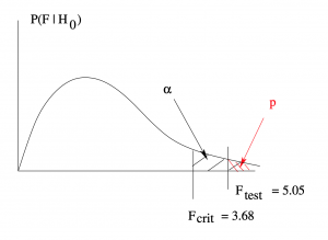
Reject $H_{0}$ .

5. Interpretation.

Using one-way ANOVA at $\alpha = 0.05$ we found that at least one of the toll roads has a different average number of employees at their interchanges. The ANOVA table is :

Source	SS	$\nu$	MS	$F$	$p$ (sig)
Between (signal)	459.18	2	229.59	5.05	$p < 0.05$
Within (error)	682.5	15	45.5
Totals	1141.68	17

We did not compute $p$ but a computer program like SPSS will.

▢

The mean of the $F_{\nu_{1},\nu_{2}}$ distribution is $\mu_{F} = \frac{\nu_{2}}{\nu_{2} - 2}$ if $\nu_{2} > 2$ . ↵
You might have heard of RMS for "root mean square". RMS = $\sqrt{\mbox{MS}} = \sqrt{{s}^{2}} = s$ . RMS is standard deviation. ↵

License

Icon for the Creative Commons Attribution-NonCommercial-ShareAlike 4.0 International License

Introduction to Applied Statistics for Psychology Students Copyright © 2022 by Gordon E. Sarty is licensed under a Creative Commons Attribution-NonCommercial-ShareAlike 4.0 International License, except where otherwise noted.

License

Share This Book