
14. Correlation and Regression
14.6 r² and the Standard Error of the Estimate of y′
Consider the deviations :
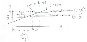
Looking at the picture we see that

Remember that variance is the sum of the squared deviations (divided by degrees of freedom), so squaring the above and summing gives:
![\[ \sum_{i=1}^{n} (y_{i} - \overline{y}_{i})^{2} = \sum_{i=1}^{n} (y^{\prime}_{i} - \overline{y}_{i})^{2} + \sum_{i=1}^{n} (y_{i} - y^{\prime}_{i})^{2} \]](https://openpress.usask.ca/app/uploads/quicklatex/quicklatex.com-6d72a77693a557e8f78ac28cda6ed283_l3.png "Rendered by QuickLaTeX.com")
(the cross terms all cancel because  is the least square solution and
  , see Section 14.6.1, below, for details). This is also a sum of squares statement:
![\[ \mbox{SS}_{T} = \mbox{SS}_{R} + \mbox{SS}_{E} \]](https://openpress.usask.ca/app/uploads/quicklatex/quicklatex.com-75797615f95c432d0f331de82965c252_l3.png "Rendered by QuickLaTeX.com")
where SS , SS
, SS and SS
 are the sum of squares — error, sum of squares — total and sum of squares — regression (explained) respectively.
Dividing by the degrees of freedom, which is  in this {\em bivariate} situation, we get:

It turns out that
![\[ r^{2} = \frac{\mbox{explained variance}}{\mbox{total variance}} = \frac{ \mbox{SS}_{R} }{ \mbox{SS}_{T} } \]](https://openpress.usask.ca/app/uploads/quicklatex/quicklatex.com-755ec04a84bafa9a82ac5cfa83824c73_l3.png "Rendered by QuickLaTeX.com")
The quantity  is called the coefficient of determination and gives the the fraction of variance explained by the model (here the model is the equation of a line). The quantity appears with many statistical models. For example with ANOVA it turns out that the “effect size” eta-squared is the fraction of variance explained by the ANOVA model[1],
  .
.
The standard error of the estimate is the standard deviation of the noise (the square root of the unexplained variance) and is given by
![\[ s_{\mbox{est}} = \sqrt{\frac{\sum (y - y^{\prime})^{2} }{n-2} } = \sqrt{\frac{\sum y^{2} - a \sum y - b \sum xy}{n-2} } \]](https://openpress.usask.ca/app/uploads/quicklatex/quicklatex.com-3d6fc96b9fb4c090d021057fbc90e584_l3.png "Rendered by QuickLaTeX.com")
Example 14.4: Continuing with the data of Example 14.3, we had
![\[ \sum y = 511 \;\;\; \sum y^{2} = 38993 \;\;\; \sum xy = 3745 \;\;\; a = 102.493 \;\;\; b = -3.622 \;\;\; n=7 \]](https://openpress.usask.ca/app/uploads/quicklatex/quicklatex.com-28c90cfe002049583c9fcca96ae0a585_l3.png "Rendered by QuickLaTeX.com")
so

▢
Here is a graphical interpretation of  :
:
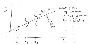
The assumption for computing confidence intervals for is that is independent of  . This is the assumption of homoscedasticity. You can think of the regression situation as a generalized one-way ANOVA where instead of having a finite number of discrete populations for the IV, we have an infinite number of (continuous) populations. All the populations have the same variance
  (and they are assumed to be normal) and
  is the pooled estimate of that variance.
14.6.1: **Details: from deviations to variances
Squaring both sides of
![\[ (y_{i} - \overline{y}_{i}) = (y^{\prime}_{i} - \overline{y}_{i}) + (y_{i} - y^{\prime}_{i}) \]](https://openpress.usask.ca/app/uploads/quicklatex/quicklatex.com-292714a4193046d48df181fd404a1064_l3.png "Rendered by QuickLaTeX.com")
and summing gives
![\[ \sum (y_{i} - \overline{y}_{i})^{2} = \sum (y^{\prime}_{i} - \overline{y}_{i})^{2} + \sum (y_{i} - y^{\prime}_{i})^{2} + \sum 2 (y^{\prime}_{i} - \overline{y})(y_{i} - y^{\prime}_{i}) \]](https://openpress.usask.ca/app/uploads/quicklatex/quicklatex.com-9fbf9ece7c701d326ac7a76c5e216355_l3.png "Rendered by QuickLaTeX.com")
Working on that cross term, using , we get

where
![\[ b = \frac{\sum (x_{i}-\overline{x})(y_{i}-\overline{y})}{\sum(x_{i}-\overline{x})^{2}} \]](https://openpress.usask.ca/app/uploads/quicklatex/quicklatex.com-a8975ae7431e60cbaceb721529045f7b_l3.png "Rendered by QuickLaTeX.com")
was used in the last line.
- In ANOVA the ``model'' is the difference of means between the groups. We will see more about this aspect of ANOVA in Chapter 17. ↵
