
8. Confidence Intervals
8.4 Proportions and Confidence Intervals for Proportions
We will now make use of the approximation of the binomial distribution by the  -distribution given in Section 7.1: Using the Normal Distribution to Approximate the Binomial Distribution. As usual, the confidence interval will switch the roles of population and sample quantities. The recipe will be laid out first, then we will connect it to what you know about the binomial distribution.
First some definitions. Let  be the number of items in a population of size
  that have a given quality. (e.g. the number of females in a population; or the number of people at the U of S wearing yellow sweaters). Then the proportion of the population having the given quality is
![\[ p = \frac{X}{N} \]](https://openpress.usask.ca/app/uploads/quicklatex/quicklatex.com-9a9141e9f50148387c97f281198145d4_l3.png "Rendered by QuickLaTeX.com")
Given a sample from the population of size  , the best estimate for
  is:
is:
![\[\hat{p} = \frac{x}{n}\]](https://openpress.usask.ca/app/uploads/quicklatex/quicklatex.com-890701c4963fa1976555f00cfcf4e39c_l3.png "Rendered by QuickLaTeX.com")
where  is the number of items in the sample having the given quality. To go along with
  we also have
![\[\hat{q} = 1 -\hat{p}\]](https://openpress.usask.ca/app/uploads/quicklatex/quicklatex.com-423973575456a2f509d2dca890eda067_l3.png "Rendered by QuickLaTeX.com")
which is is the proportion of items in the sample without the given quality.
To compute an  confidence interval for a proportion we need to compute
![\[ E = z_{\cal{C}} \sqrt{\frac{\hat{p} \hat{q}}{n}}\]](https://openpress.usask.ca/app/uploads/quicklatex/quicklatex.com-9aee5de7a1628152d17cf99032ab4dd5_l3.png "Rendered by QuickLaTeX.com")
and it must be true that both  and
and  (otherwise we need to use the binomial distribution directly).
With  , the confidence interval for a proportion is given by
![\[ \hat{p} - E < p < \hat{p} + E.\]](https://openpress.usask.ca/app/uploads/quicklatex/quicklatex.com-9ff6eec02368b373ec291f0c393fc090_l3.png "Rendered by QuickLaTeX.com")
To derive the proportions confidence interval formula we’ll begin with the sampling theory given by the binomial distribution and the corresponding -approximation. Then we’ll switch the roles of and . Let
![\[x_{\rm pop} = \frac{n}{N} X = np\]](https://openpress.usask.ca/app/uploads/quicklatex/quicklatex.com-e9e877ce4ab664760689caed86e65ccc_l3.png "Rendered by QuickLaTeX.com")
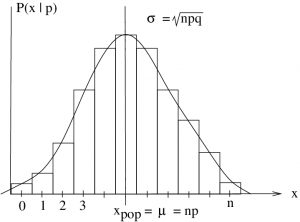
be the mean, the expected value, of that you expect to find in a sample of size randomly selected from the population with a proportion of items of interest. This is true because is also the probability of randomly selecting an item of interest (the probability of success) from the population as per what we did in Chapter 4. The binomial distribution tells you the probability of getting different numbers of items of interest in your sample given . The binomial distribution that describes our situation is shown in Figure 8.7; it has a standard deviation of  .
.
 with items of interest from a population with a proportion of items of interest. The normal distribution with the same
  and
and  is shown.
Moving to the normal approximation, we have the picture of Figure 8.8.
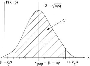 with items of interest from a population with a proportion of items of interest. The boundaries of the area follow from an inverse -transform of the -distribution to a normal distribution of mean and standard deviation ,
  .
.Figure 8.8 says :

with a (frequentist) probability of . This is our sampling theory. Divide by :

Swapping the roles of the population and sample, we arrive at the confidence interval formula :
![\[\hat{p} - z_{\cal{C}} \sqrt{\frac{\hat{p}\hat{q}}{n}} \:\: < \:\: p \:\: < \:\: \hat{p} + z_{\cal{C}}\sqrt{\frac{\hat{p}\hat{q}}{n}}.\]](https://openpress.usask.ca/app/uploads/quicklatex/quicklatex.com-2f05782dac15869d4601b346425d7626_l3.png "Rendered by QuickLaTeX.com")
Time for a worked example.
Example 8.3 : A sample of 500 nursing applications included 60 men. Find the 90% confidence interval of the true proportion of men who applied to the nursing program.
Solution : From the t Distribution Table, look up
![\[z_{\cal{C}} = 1.65\]](https://openpress.usask.ca/app/uploads/quicklatex/quicklatex.com-8aadff084931a5f36c1de75fe2956f46_l3.png "Rendered by QuickLaTeX.com")
and compute
![\[\hat{p} = \frac{x}{n} = \frac{60}{500} = 0.12\]](https://openpress.usask.ca/app/uploads/quicklatex/quicklatex.com-9e2f7bff12844fd996168799987fccb3_l3.png "Rendered by QuickLaTeX.com")
![\[\hat{q} = 1 -\hat{p} = 1 - 0.12 = 0.88\]](https://openpress.usask.ca/app/uploads/quicklatex/quicklatex.com-c6a8ccf1527433ea9e7f58b4ca5c7340_l3.png "Rendered by QuickLaTeX.com")
![\[E = z_{\alpha/2} \cdot \sqrt{\frac{\hat{p}\hat{q}}{n}} = 1.65\sqrt{\frac{(0.12) \cdot (0.88)}{500}} = 0.024. \]](https://openpress.usask.ca/app/uploads/quicklatex/quicklatex.com-06023c190c0b4ba90f612075e6141ecb_l3.png "Rendered by QuickLaTeX.com")
Then
![\[\hat{p}+E < p < \hat{p}-E\]](https://openpress.usask.ca/app/uploads/quicklatex/quicklatex.com-70cec64c78744798646941edba0d8a37_l3.png "Rendered by QuickLaTeX.com")
![\[0.12-0.024 < p < 0.12+0.024\]](https://openpress.usask.ca/app/uploads/quicklatex/quicklatex.com-7df4f082f1c9370235b49a283cb3c083_l3.png "Rendered by QuickLaTeX.com")
![\[0.096 < p < 0.144\]](https://openpress.usask.ca/app/uploads/quicklatex/quicklatex.com-b9964e1e163d04bd68cd9c9d82fdacd4_l3.png "Rendered by QuickLaTeX.com")
is the confidence interval with 90% confidence.
▢
Sample size need for a poll
Measuring proportions is what pollsters do. For example in an election you might want to know how many people will vote for liberals (items of interest) and how many will vote for conservatives (items not of interest)[1] In a news paper you might see: “The poll says that 72 of the voters will vote liberal. The poll is considered accurate to 2 percentage points 19 time out of 20.” This means that the 95 confidence interval (19/20 = 0.95) of the proportion of liberal voters is
  (note how proportions are presented as percentages in the newspaper). The error here is
  . Before the pollster starts telephoning people, she must know how many people to phone to arrive at that goal error of 2. She needs to know what the sample size needed is. In general, the minimum sample size needed to attain a goal error on a confidence interval of is
![\[n = \hat{p}\hat{q}\left( \frac{z_{\cal{C}}}{E} \right)^{2}.\]](https://openpress.usask.ca/app/uploads/quicklatex/quicklatex.com-37d2a73c78afe78e1ee6260e0b7ffd86_l3.png "Rendered by QuickLaTeX.com")
Here and  could come from a previous survey if available. If there is no such survey or if you want to be sure of ending up with an error equal to or less than a goal E, then use
  , see Figure 8.9.
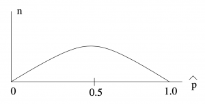
 is a quadratic formula. Substitute
  to get
  or
or  . The maximum of
  is at
is at  .
.Example 8.4 : We want to estimate, with 95 confidence, the proportion of people who own a home computer. A previous study gave an answer of 40. For a new study we want an error of 2. How many people should we poll?
Solution : From the question we have :
![\[\hat{p}=0.40, \hspace{.25in} \hat{q}=0.60\]](https://openpress.usask.ca/app/uploads/quicklatex/quicklatex.com-268cdb9be6b9590400e206ace0eb477a_l3.png "Rendered by QuickLaTeX.com")
![\[E = 0.02, \hspace{.25in} \alpha = 0.95\]](https://openpress.usask.ca/app/uploads/quicklatex/quicklatex.com-7fff5a294aa79876910ade2df7ccdcb4_l3.png "Rendered by QuickLaTeX.com")
From the t Distribution Table (or the Standard Normal Distribution Table if you think about the areas correctly) we find
![\[z_{\cal{C}} = z_{95\%} = 1.960.\]](https://openpress.usask.ca/app/uploads/quicklatex/quicklatex.com-6075a16206cf1e7ca840b3d4d208eadb_l3.png "Rendered by QuickLaTeX.com")
Therefore
![\[n = \hat{p}\hat{q}\left( \frac{z_{\alpha/2}}{E}\right)^2 = (0.40)(0.60)\left( \frac{1.96}{0.02}\right)^2 = 2304.96\]](https://openpress.usask.ca/app/uploads/quicklatex/quicklatex.com-f66a3d251d5de38a558252ab16c42f5b_l3.png "Rendered by QuickLaTeX.com")
Which we round up to a sample size of 2305 to ensure that  .
.
▢
- We assume here that there are only two parties. For the real life situation of more than two parties we need the multinomial distribution and to approximate it with a multivariate normal distribution. That is a topic for multivariate statistics but the principles are the same as what we cover here. ↵
