
8. Confidence Intervals
8.2 **Bayesian Statistics
Now that we’ve seen how easy it is to compute confidence intervals, let’s give it a proper probabilistic meaning. To extend probability from the frequentist definition to the Bayesian definition, we need Bayes’ rule. Bayes’ rule is, for events  and
and  :
:
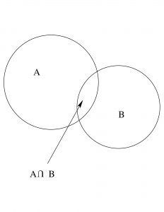
![\[ P(A \mid B) P(B) = P(B \mid A) P(A). \]](https://openpress.usask.ca/app/uploads/quicklatex/quicklatex.com-0814a0b9ac7afa7205ef378b6843a62c_l3.png "Rendered by QuickLaTeX.com")
Study Figure 8.4 to convince yourself that Bayes’ rule is true. Notice that
![\[ P(A \mid B) = \frac{P(A \cap B)}{P(B)} \]](https://openpress.usask.ca/app/uploads/quicklatex/quicklatex.com-fc5efc3a46e1b18088d15c4fc5b17ea0_l3.png "Rendered by QuickLaTeX.com")
and
![\[ P(B \mid A) = \frac{P(A \cap B)}{P(A)}. \]](https://openpress.usask.ca/app/uploads/quicklatex/quicklatex.com-616b4c6173b01e9d0925bcdac4454143_l3.png "Rendered by QuickLaTeX.com")
So, equating  from each of those two perspectives, we get Bayes’ rule.
If we let  (hypothesis) and
  (data), Bayes’ rule gives us a way to define the probability of hypothesis through
(8.2) ![\begin{equation*} P(H \mid D) = P(D \mid H)\left[ \frac{P(H)}{P(D)} \right]. \end{equation*}](https://openpress.usask.ca/app/uploads/quicklatex/quicklatex.com-3f453995ca03a5dfa431326ccae197bb_l3.png "Rendered by QuickLaTeX.com")
The quantity ![[P(H)/P(D)]](https://openpress.usask.ca/app/uploads/quicklatex/quicklatex.com-f6b5db2bb941548c7f0e712a129af87a_l3.png "Rendered by QuickLaTeX.com") is known as the prior probability of the data relative to the hypothesis and is something that can be computed in theory if probabilities are assigned in a reasonable manner. The specification of prior probabilities is a contentious issue with the Bayesian approach. Really, it represents a prior belief. The quantity
is known as the prior probability of the data relative to the hypothesis and is something that can be computed in theory if probabilities are assigned in a reasonable manner. The specification of prior probabilities is a contentious issue with the Bayesian approach. Really, it represents a prior belief. The quantity  is what sampling theory, like the central limit theorem, gives and is known as the likelihood. Finally the quantity
  is known as the posterior probability. Equation (8.2) is an expression about probability distributions as well as individual probabilities (just allow
  and
and  to vary).
If we assign ![[P(H)/P(D)] = 1](https://openpress.usask.ca/app/uploads/quicklatex/quicklatex.com-404094be24b29bf6454a6c53a14707bd_l3.png "Rendered by QuickLaTeX.com") for the prior probability then
for the prior probability then  . We can switch the roles of and ! Of course is not a probability distribution because the area under a function whose value is always 1 is infinite. The area under a probability distribution must be 1. So is an improper distribution (as a function of either or ). But note that an improper distribution times a proper distribution here gives rise to a proper distribution. With this slight of hand, we can give confidence intervals a probabilistic interpretation.
