10.4 Unpaired or Independent Sample t-Test

Gordon E. Sarty

10. Comparing Two Population Means

10.4 Unpaired or Independent Sample t-Test

In comparing the variances of two populations we have one of two situations :

Homoscedasticity : $\sigma^2_1 = \sigma^2_2$
Heteroscedasticity : $\sigma^2_1 \neq \sigma^2_2$

These terms also apply when there are more than 2 populations. They either all have the same variance, or not. This affects how we do an independent sample $t$ -test because we have two cases :

1. Variances of the two populations assumed unequal. $\sigma^2_1 \neq \sigma^2_2$ .

Then the test statistic is :

$t_{\rm test} = \frac{(\bar{x}_1 - \bar{x}_2)}{\sqrt{\frac{s^2_1}{n_1} + \frac{s^2_1}{n_2}}}$

This is the same formula as we used for the $z$ -test. To find the critical statistic we will use, when solving problems by hand, degrees of freedom

(10.2) $\begin{equation*} \nu = \min(n_{1}-1,n_{2}-1). \end{equation*}$

This choice is a conservative approach (harder to reject $H_{0}$ ). SPSS uses a more accurate

(10.3) $\begin{equation*} \nu = \frac{\left( \frac{s^2_1}{n_1} + \frac{s_2^2}{n_2} \right)^2}{\left[ \frac{\left( \frac{s^2_1}{n_1} \right)}{n_1-1} + \frac{\left( \frac{s^2_2}{n_2} \right)}{n_{2}-1} \right]} \end{equation*}$

You will not need to use Equation (10.3), only Equation (10.2). Equation (10.3) gives fractional degrees of freedom. The $t$ test statistic for this case and the degrees of freedom in Equation (10.3) is know as the Satterwaite approximation. The $t$ -distributions are strictly only applicable if $\sigma_{1} = \sigma_{2}$ . The Satterwaite approximation is an adjustment to make the $t$ -distributions fit this $\sigma_{1} \neq \sigma_{2}$ case.

2. Variances of the two populations assumed equal. $\sigma_{1} = \sigma_{2} = \sigma$ .

In this case the test statistic is:

$t_{\rm test} = \frac{(\bar{x}_1 - \bar{x}_2)}{\sqrt{\frac{(n_1-1)s^2_1 + (n_2-1)s^2_2}{n_1 + n_2 - 2}} \sqrt{\frac{1}{n_1} + \frac{1}{n_2}}}$

This test statistic formula can be made more intuitive by defining

(10.4) $\begin{equation*} s_{p} = \sqrt{\frac{(n_1-1)s^2_1 + (n_2-1)s^2_2}{n_1 + n_2 - 2}} \end{equation*}$

as the pooled estimate of the variance. $s_{p}$ is the data estimate for the common population $\sigma$ . $s_{p}^{2}$ is the weighted mean of the sample variances $s_{1}^{2}$ and $s_{2}^{2}$ . Recall the generic weighted mean formula, Equation (3.2). The weights are $\nu_{1} = n_{1}-1$ and $\nu_{2}=n_{1}-1$ ; their sum is $\nu_{1} + \nu_{2} = n_{1} - 1 + n_{2} -1 = n_{1} + n_{2} -2$ . In other words

$s_{p}^{2} = \frac{\nu_{1} s_{1}^{2} + \nu_{2} s_{2}^{2}}{\nu_{1} + \nu_{2}}$

and we can write the test statistic as

(10.5) $\begin{equation*} t_{\rm test}= \frac{(\bar{x}_1 - \bar{x}_2)}{s_{p} \sqrt{\frac{1}{n_1} + \frac{1}{n_2}}}. \end{equation*}$

See that $s_{p} \sqrt{\frac{1}{n_1} + \frac{1}{n_2}}$ is clearly a standard error of the mean.

10.4.1 General form of the t test statistic

All $t$ statistics have the form :

$t_{\rm test}= \frac{\mbox{Difference of means}}{\mbox{Standard error of the mean}} = \frac{\mbox{Signal}}{\mbox{Noise}}.$

Remember that! Memorizing complicated formulae is useless, but you should remember the basic form of a $t$ test statistic.

10.4.2 Two step procedure for the independent samples t test

We will use the $F$ test to decide whether to use case 1 or 2. SPSS uses a test called “Levine’s test” instead of the $F$ test we developed to test $H_{0}: \sigma^2_1 \neq \sigma^2_2$ . Levine’s test also produces an $F$ test statistic. It is a different $F$ than our $F$ but you interpret it in the same way. If the $p$ -value of the $F$ is high (larger than $\alpha$ ) then assume $\sigma_{1} = \sigma_{2}$ , if the $p$ -value is low (smaller than $\alpha$ ) then assume $\sigma_{1} \neq \sigma_{2}$ .

In real life, homoscedasticity is almost always assumed because the $t$ -test is robust to violations of homoscedasticity until one sample set contains twice as many, or more, data points as the other.

Example 10.4: Case 1 example.

Given the following data summary :

$s_{1}=38$

$\overline{x}_{1}=191$

$n_{1}=8$

$s_{2}=12$

$\overline{x}_{2}=199$

$n_{2}=10$

(Note that $(s_{1}=38) > (s_{2}=12)$ . If that wasn’t true, we could reverse the definitions of populations 1 and 2 so that $F_{\rm test} > 1$ .) Is $\overline{x}_1$ significantly different from $\overline{x}_2$ ? That is, is $\mu_1$ different from $\mu_2$ ? Test at $\alpha=0.05$ .

Solution :

So the question is to decide between

$H_{0}: \mu_{1} = \mu_{2} \hspace{.5in} H_{1}: \mu_{1} \neq \mu_{2}$

a two-tailed test. But before we can test the question, we have to decide which $t$ test statistic to use: case 1 or 2. So we need to do two hypotheses tests in a row. The first one to decide which $t_{\rm test}$ statistic to use, the second one to test the hypotheses of interest given above.

Test 1 : See if variances can be assumed equal or not.

1. Hypothesis.

$H_0: \sigma^2_1 = \sigma^2_2\hspace{.25in} H_1: \sigma^2_1 \neq \sigma^2_2$

(Always use a two-tailed hypothesis when using the $F$ test to decide between case 1 and 2 for the $t$ test statistic.)

2. Critical statistic.

$F_{\rm crit} = F_{\alpha/2, \nu_1, \nu_2} = F_{0.05/2, 7, 9} = F_{0.025},7 ,9 = 4.20$

(from the F Distribution Table)

(Here we used $\alpha$ given for the $t$ -test question. But that is not necessary. You can use $\alpha = 0.05$ in general; the consequence of a type I error here is small because the $t$ -test is robust to violations of the assumption of homoscedasticity.)

3. Test statistic.

$F_{\rm test} = F_{7, 9} = \frac{s^2_1}{s^2_2} = \frac{38^2}{12^2} = 10.03$

4. Decision.

$10.03 > 4.20$ ( $F_{\rm test} > F_{\rm crit}$ — drawing a picture would be a safe thing to do here as usual) so reject $H_{0}$ .

5. Interpretation.

Assume the variances are unequal, $\sigma_{1}^{2} \neq \sigma_{2}^{2}$ , and use the $t$ test statistic of case 1.

Test 2 : The question of interest.

1. Hypothesis.

$H_0: \mu_1 = \mu_2\hspace{.25in}H_1: \mu_1 \neq \mu_2$

2. Critical statistic.

From the t Distribution Table, with $\nu =\min(n_{1}-1,n_{2}-1) = \min(8-1, 10-1) \min(7,9) = 7$ , and a two-tailed test with $\alpha = 0.05$ we find

$t_{\rm crit} = \pm 2.365$

3. Test Statistic.

$\begin{eqnarray*} t & = & \frac{(\bar{x}_1 - \bar{x}_2)}{\sqrt{\frac{s^2_1}{n_1} + \frac{s^2_2}{n_2}}} \\ & = & \frac{(191 - 199)}{\sqrt{\frac{38^2}{8} + \frac{12^2}{10}}} = -0.57 \end{eqnarray*}$

The $p$ -value may be estimated from the t Distribution Table using the procedure given in Chapter 9: from the t Distribution Table, $\nu = 7$ line, find the values that bracket 0.57. There are none, the smallest value is 0.711 corresponding to $\alpha = 0.50$ . So all we can say is $p > 0.50$ .

4. Decision.

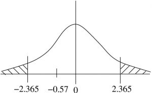
$t_{\rm test} = -0.57$ is not in the rejection region so do not reject $H_{0}$ . The estimate for the $p$ -value confirms this decision.

5. Interpretation.

There is not enough evidence, at $\alpha = 0.05$ with the independent sample $t$ -test, to conclude that the means of the populations are different.

▢

Example 10.5 (Case 2 example) :

The following data seem to show that private nurses earn more than government nurses :

Private Nurses Salary

Government Nurses Salary

$\bar{x}_1 = 26,800$

$\bar{x}_2 = 25,400$

$s_1 = 600$

$s_2 = 450$

$n_1 = 10$

$n_2 = 8$

Testing at $\alpha=0.01$ , do private nurses earn more than government nurses?

Solution :

First confirm, or change, the population definitions so that $s_{1}^{2} > s_{2}^{2}$ . This is already true so we are good to go.

Test 1 : See if variances can be assumed equal or not. This is a test of $H_{0}: \sigma_{1}^{2} = \sigma_{2}^{2}$ vs. $H_{1}: \sigma_{1}^{2} \neq \sigma_{2}^{2}$ . After the test we find that we believe that $\sigma_{1}^{2} = \sigma_{2}^{2}$ at $\alpha = 0.05$ . So we will use the case 2, equal variances, $t$ -test formula for test 2, the test of interest.

Test 2 : The question of interest.

1. Hypothesis.

$H_{0}: \mu_{1} \leq \mu_{2}$

$H_{1}: \mu_{1} > \mu_{2}$

(Note how $H_{1}$ reflects the face value of the data, that private nurses appear to earn more than government nurses in the population — it is true in the samples.)

2. Critical statistic.

Use the t Distribution Table, one-tailed test, $\alpha = 0.01$ (column) and $\nu = n_{1} + n_{2} -2 = 10+8-2=16$ to find

$t_{\rm crit} = 2.583$

3. Test statistic.

$\begin{eqnarray*} t_{\rm test} &=& \frac{(\bar{x}_1 - \bar{x}_2)}{\sqrt{\frac{(n_1-1)s^2_1 + (n_2-1)s^2_2}{n_1+n_2-2}} \sqrt{\frac{1}{n_1} + \frac{1}{n_2}}} \\ t_{\rm test} &=& \frac{(26,800 - 25,400)}{\sqrt{\frac{(10-1)600^2 + (8-1)450^2}{10+8-2}} \sqrt{\frac{1}{10} + \frac{1}{8}}} \\ t_{\rm test} &=& \frac{1400}{\sqrt{\frac{(9)(360000) + (7)(202500)}{16}}\sqrt{0.1+0.125}} \\ t_{\rm test} &=& \frac{1400}{\sqrt{\frac{3240000 + 1417500}{16}} \sqrt{0.225}} \\ t_{\rm test} &=& \frac{1400}{(\sqrt{291093.75})(\sqrt{0.225})} = 5.47 \end{eqnarray*}$

To estimate the $p$ -value, look at the $\nu = 16$ line in the t Distribution Table to see if there are a pair of numbers that bracket $t_{\rm test}=5.47$ . They are all smaller than 5.47 so $p$ is less than the $\alpha$ associated with the largest number 2.921 whose $\alpha$ is 0.005 (one-tailed, remember). So $p < 0.005$ .