9.2 z-Test for a Mean

Gordon E. Sarty

9. Hypothesis Testing

9.2 z-Test for a Mean

This is our first hypothesis test. Use it to test a sample’s mean when :

The population $\sigma$ is known.
Or When $n \geq 30$ , in which case use $\sigma = s$ in the test statistic formula.

The possible hypotheses are as given in the table you saw in the previous section (one- and two-tailed versions):

Two-Tailed Test

Right-Tailed Test

Left-Tailed Test

$H_{0}$ : $\mu = k$

$H_{0}$ : $\mu \leq k$

$H_{0}$ : $\mu \geq k$

$H_{1}$ : $\mu \neq k$

$H_{1}$ : $\mu > k$

$H_{1}$ : $\mu < k$

In all cases the test statistic is

(9.1) $\begin{equation*} z_{\rm test} = \frac{\bar{x} - k}{(\sigma/\sqrt{n})}. \end{equation*}$

In real life, we will never know what the population $\sigma$ is, so we will be in the second situation of having to set $\sigma = s$ in the test statistic formula. When you do that, the test statistic is actually a $t$ test statistic as we’ll see. So taking it to be a $z$ is an approximation. It’s a good approximation but SPSS never makes that approximation. SPSS will always do a $t$ -test, no matter how large $n$ is. So keep that in mind when solving a problem by hand versus using a computer.

Let’s work through a hypothesis testing example to get the procedure down and then we’ll look at the derivation of the test statistic of Equation (9.1).

Example 9.2 : A researcher claims that the average salary of assistant professors is more than $42,000. A sample of 30 assistant professors has a mean salary of $43,260. At $\alpha = 0.05$ , test the claim that assistant professors earn more than $42,000/year (on average). The standard deviation of the population is $5230.

Solution :

1. Hypothesis :

$H_{0} :\mu \leq 42,000$

$H_{1} : \mu > 42,000$ (claim)

(This is a right-tailed test.)

2. Critical Statistic.

Method (a) : Find $z$ such that $A(z) = 0.45$ from the Standard Normal Distribution Table: $z_{\rm critical} = 1.65$ ; or

Method (b) : Look up $z$ in the t Distribution Table corresponding to one tail $\alpha = 0.05$ (column), and read the last ( $z$ ) line: $z_{\rm critical} = 1.645.$

Method (b) is the recommended method not only because it is faster but also because the procedure for the upcoming $t$ -test will be the same for the $z$ -test.

3. Test Statistic.

$z_{\rm test} = \frac{\bar{x} - k}{\left( \frac{\sigma}{\sqrt{n}}\right)} = \frac{43260 - 42000}{\left( \frac{5230}{\sqrt{30}}\right)} = 1.32$

4. Decision.

Draw a picture so you can see the critical region :

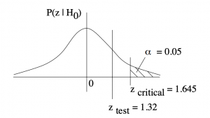
So $z$ is in the non-critical region: Do not reject $H_{0}$ .

5. Interpretation.

There is not enough evidence, from a $z$ -test at $\alpha = 0.05$ , to support the claim that professors earn more than $42,000/year on average.

▢

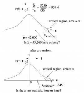
So where does Equation (9.1) come from? It’s an application of the central limit theorem! In Example 9.2, $\bar{x} = 43,260$ , $n = 30$ , $\sigma = 5230$ and $k = 42,000$ on the null hypothesis of a right-tailed test. The central limit theorem says that if $H_{0}$ is true then we can expect the sample means, $\bar{x}$ to be distributed as shown in the top part of Figure 9.1. Setting $\alpha = 0.05$ means that if the actual sample mean, $\bar{x}$ ends up in the tail of the expected (under $H_{0}$ ) distribution of sample means then we consider that either we picked an unlucky 5 $\%$ sample or the null hypothesis, $H_{0}$ , is not true. In taking that second option, rejecting $H_{0}$ , we are willing to live with the 0.05 probability that we made a wrong choice — that we made a type I error.

Figure 9.1: Derivation of the $z$ test statistic.

Referring to Figure 9.1 again, $z_{\rm critical} = 1.645$ on the lower picture defines the critical region of area $\alpha = 0.05$ (in this case). It corresponds to a value $\bar{x}_{\rm critical}$ on the upper picture which also defines a critical region of area $\alpha = 0.05$ . So comparing $\bar{x}$ to $\bar{x}_{\rm critical}$ on the original distribution of sample means, as given by the sampling theory of the central limit theorem, is equivalent, after $z$ -transformation, to comparing $z_{\rm test}$ with $z_{\rm critical}$ . That is, $z_{\rm test}$ is the $z$ -transform of the data value $\bar{x}$ , exactly as given by Equation (9.1).

One-tailed tests

From a frequentist point of view, a one-tailed test is a a bit of a cheat. You use a one-tailed test when you know for sure that your test value or statistic is greater than (or less than) the null hypothesis value. That is, for the case of means here, you know for sure that the mean of the population, if it is different from the null hypothesis mean, if greater than (or less than) the null hypothesis mean. In other words, you need some a priori information (a Bayesian concept) before you do the formal hypothesis test.

In the examples that we will work through in this course, we will consider one-tailed tests when they make logical sense and will not require formal a priori information to justify the selection of a one-tailed test. For a one-tail test to make logical sense, the alternate hypothesis, $H_{1}$ , must be true on the face value of the data. That is, if we substitute the value of $\bar{x}$ for $\mu$ into the statement of $H_{0}$ (for the test of means) then it should be a true statement. Otherwise, $H_{1}$ is blatantly false and there is no need to do any statistical testing. In any statistical test, $H_{1}$ must be true at face value and we do the test to see if $H_{1}$ is statistically true. Another way tho think about this is to think of $\bar{x}$ as a fuzzy number. As a sharp number a statement like “ $\bar{x} > k$ ” may be true, but $\bar{x}$ is fuzzy because of $s$ (think $\bar{x} = \bar{x} \pm s$ to get the fuzzy number idea). So “ $\bar{x} > k$ ” may not be true when $\bar{x}$ is considered to be a fuzzy number^[1]

When we make our decision (step 4) we consider the equality part of the $H_{0}$ statement in one-tailed tests. This equality is the strict $H_{0}$ under all circumstances but we use $\geq$ or $\leq$ is $H_{0}$ statements simply because they are the logical opposite of $<$ or $>$ in the $H_{1}$ statements. So people may have an issue with this statement of $H_{0}$ but we will keep it because of the logical completeness of the $H_{0}$ , $H_{1}$ pair and the fact that hypothesis testing is about choosing between two well-defined alternatives.

p-Value

The critical statistic defines an area, a probability, $\alpha$ that is the maximum probability that we are willing to live with for making a type I error of incorrectly rejecting $H_{0}$ . The test statistic also defines an analogous area, called $p$ or the $p$ -value or (by SPSS especially) the significance. The $p$ -value represents the best guess from the data that you will make a type I error if you reject $H_{0}$ . Computer programs compute $p$ -values using CDFs. So when you use a computer (like SPSS) you don’t need (or usually have) the critical statistic and you will make your decision (step 4) using the $p$ -value associated with the test statistic according to the rule:

$\mbox{If } p\leq \alpha \mbox{ reject } H_{0}.$

$\mbox{If } p> \alpha \mbox{ do not reject } H_{0}.$

The method of comparing test and critical statistics is the traditional approach, popular before computers because is is less work to compute the two statistics than it is to compute $p$ . When we work problem by hand we will use the traditional approach. When we use SPSS we will look at the $p$ -value to make our decision. To connect the two approaches pedagogically we will estimate the $p$ -value by hand for a while.

Example 9.3 : Compute the $p$ -value for $z{\rm test} = 1.32$ of Example 9.2.

Solution : This calculation can happen as soon as you have the test statistic in step 3. The first thing to do is to sketch a picture of the $p$ -value so that you know what you are doing, see Figure 9.2.

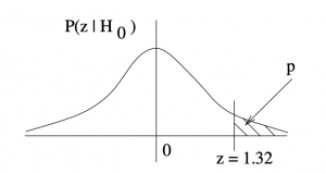Figure 9.2 : The $p$ -value associated with $z_{\rm test} = 1.32$ in a one-tail test.

Using the Standard Normal Distribution Table to find the tail area associated with $z{\rm test} = 1.32$ , we compute :

$\begin{eqnarray*} p(z_{\rm test}) & = & 0.5 - A(z_{\rm test}) \\ &=& 0.5 - 0.4066 = 0.034 \end{eqnarray*}$

That is $p = 0.0934$ . Since $(p = 0.0934) > (\alpha = 0.05)$ , we do not reject $H_{0}$ in our decision step (step 4).

▢

When using the Standard Normal Distribution Table to find $p$ -values for a given $z$ you compute).

For two-tailed tests: $p(z) = 2(0.5 - A(z))$ . See Figure 9.3.
For one-tailed tests: $p(z) = 0.5 - A(z)$ (as in Example 9.3)^[2].

Don’t try to remember these formula, draw a picture to see what the situation is.

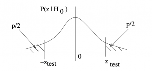Figure 9.3 : The $p$ -value associated with a two-tailed $z_{\rm test}$ . Since $\alpha$ is defined by, $\pm z_{\rm critical}$ , $p$ is defined by $\pm z_{\rm test}$ .

9.2.1 What p-value is significant?

By culture, psychologists use $\alpha = 0.05$ to define the decision point for when to reject $H_{0}$ . In that case, if $p < 0.05$ then it means that the data (the test statistic) indicates there is less than a 5% chance that the result is a statistical fluke; that there is less than a 5% chance that the decision is a Type I error. So, in this course, we assume that $\alpha = 0.05$ unless $\alpha$ is otherwise given explicitly for pedagogical purposes. The choice of $\alpha = 0.05$ is actually fairly lax and has led to the inability to reproduce psychological experiments in many cases (about 5% of course). The standards in other scientific disciplines can be different. In particle physics experiments, for example, $p < 0.003$ is referred to as “evidence” for a discovery and they must have $p < 0.0000006$ before an actual discovery, like the discovery of the Higgs boson, is announced. With z test statistics, $\alpha = 0.003$ represents the area in the tails of the $z$ distribution 3 standard deviations, or $3 \sigma$ , from the mean. The value $\alpha = 0.0000006$ represents tail area $5 \sigma$ , from the mean. So you may hear physicists saying that they have “5 sigma” evidence when they announce a discovery.

Fuzzy numbers can be treated rigorously in a mathematical sense. See, e.g. Kaufmann A, Gupta MM, Introduction to fuzzy arithmetic: theory and applications, Van Nostrand Reinhold Co., 1991. ↵
Of course substitute $-z$ in the formula for a left tail test. ↵

License

Icon for the Creative Commons Attribution-NonCommercial-ShareAlike 4.0 International License

Introduction to Applied Statistics for Psychology Students Copyright © 2022 by Gordon E. Sarty is licensed under a Creative Commons Attribution-NonCommercial-ShareAlike 4.0 International License, except where otherwise noted.

9.2.1 What p-value is significant?

License

Share This Book