
9. Hypothesis Testing
9.5 Chi Squared Test for Variance or Standard Deviation
The possible hypothesis pairs are, for variance :
| Two-tailed Test | Right-tailed Test | Left-tailed Test |
 |
 |
 |
 |
 |
 |
For standard deviation we use the square roots of everything :
| Two-tailed Test | Right-tailed Test | Left-tailed Test |
 |
 |
 |
 |
 |
 |
Note that we did not square root  . This is because we are using to stand in for whatever number. That number from
  will appear in our formulae as either
  or
or  depending on the set up. Generally we will work with variance as we work through the problem and convert to standard deviation only in the last interpretation step if required by the wording of the question.
The new test statistic is :
![\[\chi^{2}_{\rm test} = \frac{(n-1)s^2}{\sigma^2}\]](https://openpress.usask.ca/app/uploads/quicklatex/quicklatex.com-ebb9ddb267abf7bbb6743b143c6116f9_l3.png "Rendered by QuickLaTeX.com")
where  comes from the sample and comes from the number in . The degrees of freedom associated with the test statistic (for finding the critical statistic) is
  . There is no mystery where this test statistic came from — this is just how
  as a probability distribution is defined. So, for this test to be valid, the population must be normally distributed. The test here is not very robust to violations of that assumption because there is no normalizing intermediate central limit theorem here.
The critical regions on the distribution will appear as shown in Figure 9.5.
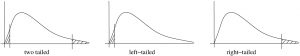 tests of variance. In the two-tailed situation the tail areas are equal.
Let’s work through an example of each hypotheses pair case. In all of the examples we assume that the population is normally distributed.
Example 9.6 : An instructor wishes to see whether the variance in scores of the 23 students in her class is less than the variance of the population. The variance of the class is 198. is there enough evidence to support the claim that the variation of the students is less than the population variance  at
at  ?
?
Solution :
1. Hypotheses.
![\[ H_{0}: \sigma^2 \geq 225 \hspace{.25in} H_{1}: \sigma^{2} < 225 \]](https://openpress.usask.ca/app/uploads/quicklatex/quicklatex.com-d67d2a70c1afe276158e4d542def1b64_l3.png "Rendered by QuickLaTeX.com")
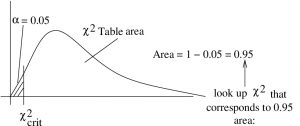
2. Critical statistic.
Refer to Figure 9.6 as we get the critical statistic from the Chi-squared Distribution Table. As we see in that figure, we must look in the column that corresponds to a right tail area of 0.95. The row we need is for  . With that information we find
  .
.
 tests of variance. In the two-tailed situation the tail areas are equal.
3. Test statistic.
The values we need for the test statistic are  (from ),
  and
and  from the information in the problem. So :

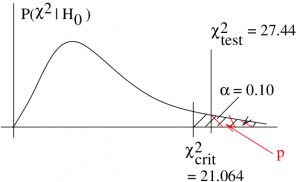
At this point we can also estimate the  value from the Chi-squared Distribution Table. The value is the area under the distribution with
  to the left of
  . In the row of the Chi-squared Distribution Table (in general use the closest
  if your particular value is not in the Chi-squared Distribution Table) hunt down the test statistic value of 19.38. You won’t find it but you can bracket it with values higher and lower than 19.38. Those numbers are 14.042 which has a right tail area of 0.90 (and so a left tail area of 0.10) and 30.813 which has a right tail area of 0.10 (and so a left tail area of 0.90). Recall that the
  in the column headings of the Chi-squared Distribution Table refers to right tail areas. So, considering the left tail areas we know that
  since
since  for the relevant values.
4. Decision.
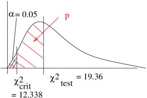
Since  doesn’t fall in the rejection region, do not reject . We come to the same conclusion with our -value estimate:
![\[ (0.10 < p < 0.90) > (\alpha = 0.05) \]](https://openpress.usask.ca/app/uploads/quicklatex/quicklatex.com-77cc05ee0c0948336d19aa27d93585d0_l3.png "Rendered by QuickLaTeX.com")
5. Interpretation.
There is not enough evidence, at with a test, to support the claim that the variation in test scores of the class is less than 225.
▢
Example 9.7 : A hospital administrator believes that the standard deviation of the number of people using out-patient surgery per day is greater than eight. A random sample of 15 days is selected. The data are shown below. At  is there enough evidence to support the administrator’s claim?

Solution :
0. Data reduction.
We’ll introduce a step 0 when it looks like we should do some preliminary calculations with or data. In this case we should enter the dataset into our calculations and determine . We find  .
.
1. Hypotheses.
![\[ H_0: \sigma^2 \leq 64 \hspace{.25in} H_1: \sigma^2 > 64 \mbox{ (claim)} \]](https://openpress.usask.ca/app/uploads/quicklatex/quicklatex.com-934182a7646f24a4e5dd7e3c7e56b521_l3.png "Rendered by QuickLaTeX.com")
Note conversion to  right away.
2. Critical statistic.
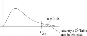
In the  line and
  column of the Chi-squared Distribution Table, look up
3. Test statistic.

To estimate the value, find the bracketing values of  in the
  line of the Chi-squared Distribution Table. They are : 26.119 (
 ) and 29.141 (
 ), so
), so  .
.
4. Decision.
Reject since is in the rejection region. Our estimate of leads to the same conclusion :
![\[ (0.010 < p < 0.025) < (\alpha = 0.10) \]](https://openpress.usask.ca/app/uploads/quicklatex/quicklatex.com-3b66b764a84f9f07ae49215eb0f41bad_l3.png "Rendered by QuickLaTeX.com")
5. Interpretation.
There is enough evidence, at with a test, to support the claim that the standard deviation is greater than 8. (Note how we convert to a statement about standard deviation after working through the problem using variances.)
▢
Example 9.8 : A cigarette manufacturer wishes to test the claim that the variance of the nicotine content of its cigarettes is 0.644. Nicotine content is measured in milligrams, assume that it is normally distributed. A sample of 20 cigarettes has a standard deviation of 1.00 kg. At , is there enough evidence to reject the manufacturer’s claim?
Solution :
1. Hypotheses.
![\[ H_{0}: \sigma^{2} = 0.644 \mbox{ (claim)} \hspace{.25in} H_{1}: \sigma^{2} \neq 0.64 \]](https://openpress.usask.ca/app/uploads/quicklatex/quicklatex.com-ea17455cd59e89a8cfc2ea551c5ca2b7_l3.png "Rendered by QuickLaTeX.com")
2. Critical statistic.
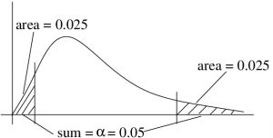
Referring to Figure 9.7, we see that we need two  values, one with a tail area of 0.025 and the other with a tail area of 1 – 0.025 = 0.975. From the Chi-squared Distribution Table in the
  line find
  from the
  column and
  from the
  column.
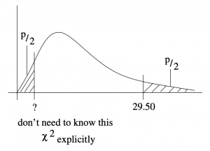
3. Test statistic.

To estimate the value find the bracketing value of  in the
  row, They are 27.204 (
 ) and 30.144 (
 ). The
  are right tail areas, which is ok, but we need to multiply them by 2 because those right tail areas represent
  as shown in Figure 9.8. So
  .
.
 associated with the test statistic (29.50 here) in a two tail test.
4. Decision.
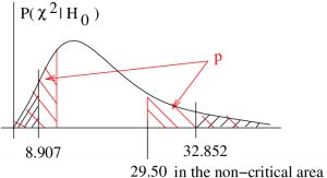
Do not reject . The estimate value leads to the same conclusion :
![\[ (0.10 < p < 0.20) > (\alpha = 0.05) \]](https://openpress.usask.ca/app/uploads/quicklatex/quicklatex.com-e591cff3ceefffc2db7dafe5c929974f_l3.png "Rendered by QuickLaTeX.com")
5. Interpretation.
There is not enough evidence, at with a test, to reject the manufacturer’s claim that the variance of the nicotine content of the cigarettes is equal to 0.644.
Notice, with the claim on , that failing to reject does not provide any evidence that is true. We just have the weaker conclusion that we couldn’t disprove it. Such is the double negative nature of the logic behind hypothesis testing that arises where we don’t assign probabilities to hypothesis.
▢
