
14. Correlation and Regression
14.8 SPSS Lesson 11: Linear Regression
Open “Hypertension.sav” from the Data Sets:
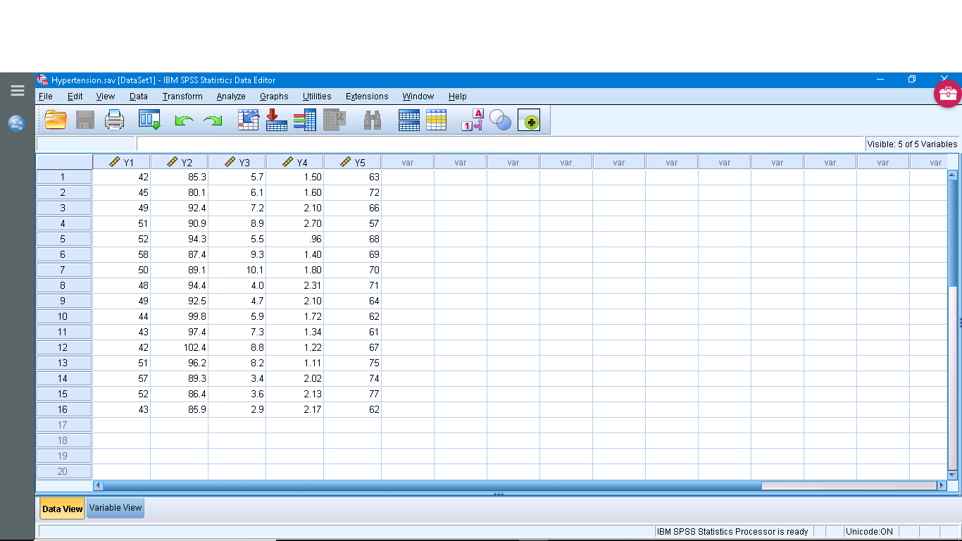
This dataset has a number of variables having to do with a study that is looking for a way to predict injury on the basis of strength. So  is the dependent (
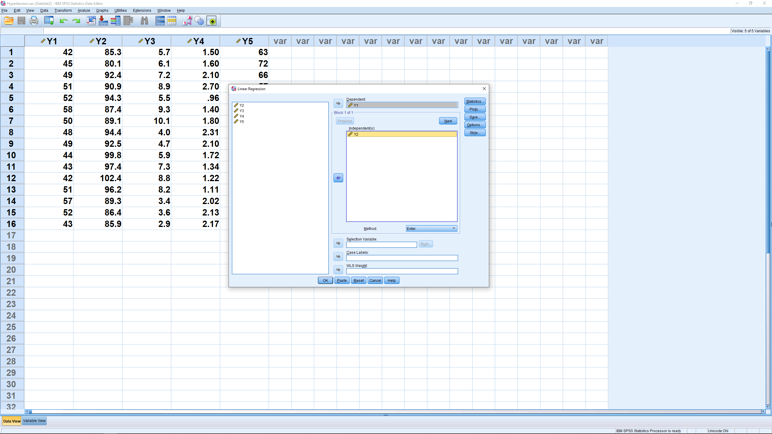
 ) variable. To get one independent variable, we’ll arbitrarily pick
  as our independent variable
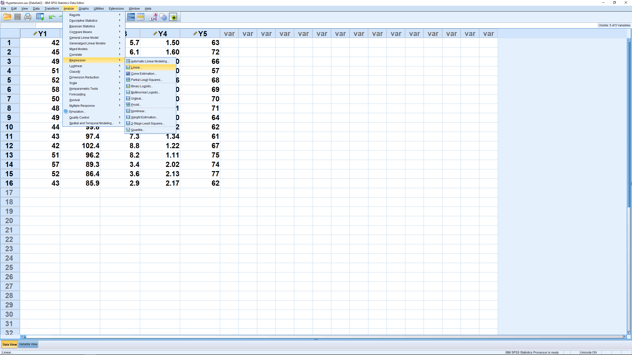
  . Next pick Analyze → Regression → Linear,
and move the independent and dependent variables into the right slots :
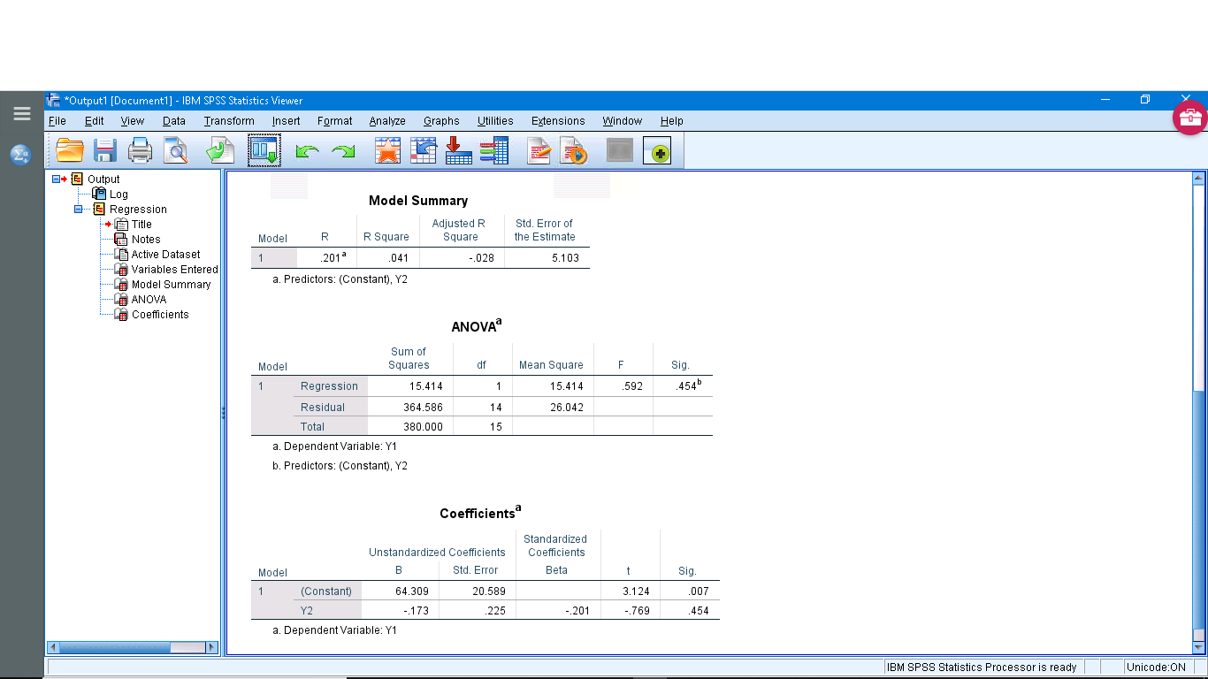
You can look through the submenus if you like but they primarily give options for multiple regression and require the consideration of the independent variable as a vector instead of as a number — this elevation of data from a number to a vector is the basis of multivariate statistics so we’ll leave that for now. Running the analysis produces four output tables. You can ignore the “Variables Entered/Removed” table (it is for advanced multiple regression analysis). The other tables show :
The “Model Summary” gives  and
and  plus
plus  and
and  that we’ll discuss when we look at multiple regression. The ANOVA table gives information about the significance of (and therefore of the overall significance of the regression). We used
  to test the significance of . You can recover the test statistic from
  in the ANOVA table;
  . Here
  so the model fit is not significant (do not reject
  ). Even though the fit is not significant, the regression can still be done and this is reported in the last output table. The coefficients are reported in the B column. They are called Unstandardized Coefficients because the data, and , have not been
  -transformed. The first line gives the intercept (
 or
or  ), the second line the slope (
 or
or  ) so
) so

For each of the two regression coefficients, a standard error can be computed, along with confidence intervals for the coefficients, and the significance of the coefficients (H :
:  ) tested with a test statistic. We haven’t covered that aspect of linear regression but we can see the standard errors, test statistics and associated
  values in the “Coefficients” output table. Here , the intercept, is significant while the slope, is not. The last thing to notice is Beta in the Standardized Coefficients column. Imagine that we -transform our variables and to
  and
and  and then did a linear regression on the -transformed variables. Then the result would be

In this case the regression is still insignificant, -transforming can’t change that. There is no intercept in this case because the average of each of -transformed variables is zero and this leads to an intercept of zero.
Finally, let’s see how we can plot the regression line. Generate a scatterplot and then double click on the plot and then click on the little icon that shows a line through scatterplot data :

and
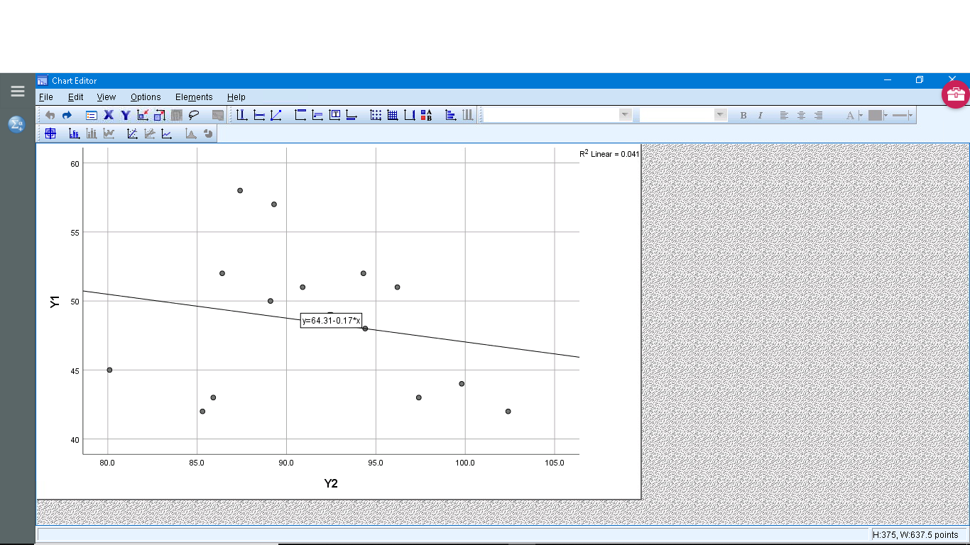
The equation of the regression line is computed instantly and is plotted.
