9.3 t-Test for Means

Gordon E. Sarty

9. Hypothesis Testing

9.3 t-Test for Means

Hypothesis testing for means for sample set sizes in $n<30$ where $s$ is used as an estimate for $\sigma$ is the same as for $n \geq 30$ except that $t$ and not $z$ is the test statistic^[1]. Specifically, the test statistic is

$t_{\rm test} = \frac{\bar{x} - k}{s/\sqrt{n}}$

for $k$ from any of the hypotheses listed in the table you saw in the previous section (one- and two-tailed versions):

Two-Tailed Test

Right-Tailed Test

Left-Tailed Test

$H_{0}$ : $\mu = k$

$H_{0}$ : $\mu \leq k$

$H_{0}$ : $\mu \geq k$

$H_{1}$ : $\mu \neq k$

$H_{1}$ : $\mu > k$

$H_{1}$ : $\mu < k$

The critical statistic is found in the t Distribution Table with the degrees of freedom $\nu = n-1$ .

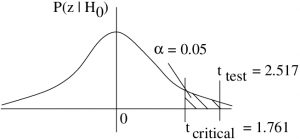
Example 9.4 : A physician claims that joggers, maximal volume oxygen uptake is greater than the average of all adults. A sample of 15 joggers has a mean of 40.6 ml/kg and a standard deviation of 6 ml/kg. If the average of all adults is 36.7 ml/kg, is there enough evidence to support the claim at $\alpha = 0.05$ ?

1. Hypothesis.

$H_{0} : \mu \leq 36.7$

$H_{1} : \mu > 36.7$ (claim)

2. Critical statistic.

In the t Distribution Table, find the column for one-tailed test at $\alpha = 0.05$ and the line for degrees of freedom $\nu = n-1 = 14$ . With that find

$t_{\rm critical} = 1.761$

3. Test statistic.

$t_{\rm test} = \frac{\bar{x} - k}{s/\sqrt{n}}$

To compute this we need : $\bar{x} = 40.6$ , $s= 6$ and $n = 15$ from the problem statement. From the hypothesis we have $k = 36.7$ . So

$t_{\rm test} = \frac{40.6 - 36.7}{\left( 6/ \sqrt{15}\right)} = 2.517$

At this point we can estimate the $p$ -value using the t Distribution Table, which doesn’t have as much information about the $t$ -distribution as the Standard Normal Distribution Table has about the $z$ -distribution, so we can only estimate. The procedure is: In the $\nu = 14$ row, look for $t$ values that bracket $t _{\rm test} = 2.517$ . They are 2.145 (with $\alpha = 0.025$ in the column heading for one-tailed tests) and 2.624 (associated with a one-tail $\alpha = 0.01$ ).

So,

$0.010 < p < 0.025$

is our estimate^[2] for $p$ .

4. Decision.

Reject $H_{0}$ . We can also base this decision on our $p$ -value estimate since :

$(0.010 < p < 0.025) < (\alpha = 0.05)$

5. Interpretation.

There is enough evidence to support the claim that the joggers’ maximal volume oxygen uptake is greater than 36.7 ml/kg using a $t$ -test at $\alpha = 0.05$ .

▢

Fine point. When we use $s$ in a $t$ (or $z$ test) as an estimate for $\sigma$ , we are actually assuming that distribution of sample means is normal. The central limit theorem tells us that the distribution of sample means is approximately normal so generally we don’t worry about this restriction. If the population is normal then the distribution of sample means will be exactly normal. Some stats texts state that we need to assume that the population is normal for a $t$ -test to be valid. However, the central limit theorem’s conclusion guarantees that the $t$ -test is robust to violations of that assumption. If the population has a very wild distribution then $s$ may be bad estimate for $\sigma$ because the distribution of sample $s$ values will not follow the $\chi^2$ distribution. The chance if this happening becomes smaller the larger the $n$ , again by the central limit theorem.

Origin of the $t$ -distribution

We can easily define the $t$ -distribution via random variables associated with the following stochastic processes. Let :

$\begin{eqnarray*} Z & = & \mbox{ a random variable with a $z$-distribution} \\ X & = & \mbox{ a random variable with a $\chi^{2}$ distribution with $\nu$ degrees of freedom.} \end{eqnarray*}$

Then the random variable

$T = \frac{Z}{X}$

is a random variable that follows a $t$ -distribution with $\nu$ degrees of freedom.

Again, SPSS applies the $t$ -test, uses $s$ directly, for any sample size. ↵
If you know how to interpolate then you can find a single value for $p$ . ↵

License

Icon for the Creative Commons Attribution-NonCommercial-ShareAlike 4.0 International License

Introduction to Applied Statistics for Psychology Students Copyright © 2022 by Gordon E. Sarty is licensed under a Creative Commons Attribution-NonCommercial-ShareAlike 4.0 International License, except where otherwise noted.

License

Share This Book