5.3 Normal Distribution

Gordon E. Sarty

5. The Normal Distributions

5.3 Normal Distribution

Let us now take a detailed look at the normal distribution and learn how to apply it to probability problems (in sampling theory) and statistical problems. Its formula (which you will never have to use because we have tables and SPSS) is again:

(5.28) $\begin{equation*} P(x) = \frac{e^{-(x-\mu)^2/2\sigma^2}}{\sigma \sqrt{2\pi}} \end{equation*}$

The factor $\sigma \sqrt{2\pi}$ is a normalization factor that ensures that the area under the whole curve is one:

$\int P(x) \: dx = 1.$

Without that factor we just have a bell-shaped curve ^[1] with the area under the curve equal to one we have a probability function since the total probability is one. For those with a bad math background, the letters in Equation (5.28) are: $e = 2.718 \ldots$ ^[2], $\pi = 3.1415 \ldots$ ^[3], $\mu$ = mean and $\sigma$ = standard deviation of the normal distribution. The normal distribution’s shape is as shown in Figure 5.2.

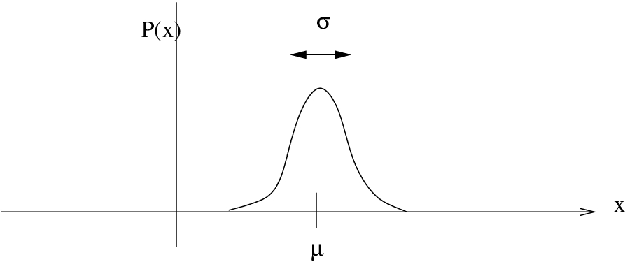
Figure 5.2: The normal distribution. It is a bell-shaped curve with its mode (= mean and median because it’s symmetric, $\mu_{3} = 0$ ) centred on its mean $\mu$ . On the left is a distribution with a large $\sigma^{2}$ and on the right one with a smaller $\sigma^{2}$ .

To work with normal distribution, in particular so we can use the Standard Normal Distribution Table and the t Distribution Table in the Appendix, we need to transform it to the standard normal distribution using the $z$ -transform. We need to transform $P(x)$ , which has a mean $\mu$ and standard deviation $\sigma$ to $P(z)$ which has a mean of 0 and a standard deviation of 1. Recall the definition of the $z$ -transform:

$z = \frac{x - \mu}{\sigma}$

applying this to $P(x)$ gives

(5.29) $\begin{equation*} P(z) = \frac{P(x) - \mu}{\sigma}. \end{equation*}$

If we substitute Equation (5.28) into Equation (5.29) and do the algebra we get :

(5.30) $\begin{equation*} P(z) = \frac{e^{-z^{2}/2}}{\sqrt{2 \pi}}. \end{equation*}$

Equation (5.30) defines the standard normal distribution, or as we’ll call it, the $z$ -distribution.
Areas under $P(z)$ are given in the Standard Normal Distribution Table in the Appendix.

5.3.1 Computing Areas (Probabilities) under the standard normal curve

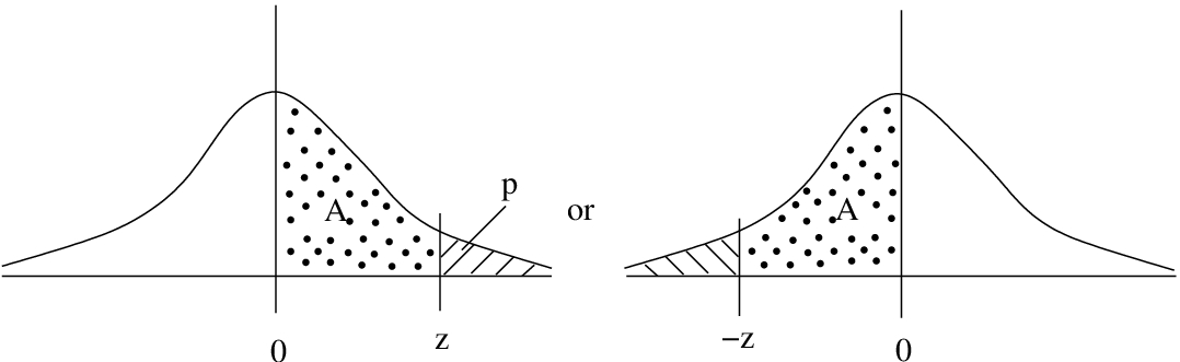
Here we learn how to use the Standard Normal Distribution Table to get probabilities associated with any old area under the normal curve that we can dream up. The general layout of areas under the $z$ -distribution is shown in Figures 5.3 and 5.4.

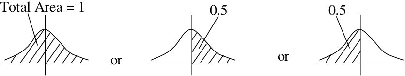Figure 5.3 : The $z$ -distribution is a probability distribution (total area = 1) and symmetric, so the area on either side of the mean (which is 0) is a half. You will need to remember this information as you calculate areas using the Standard Normal Distribution Table.

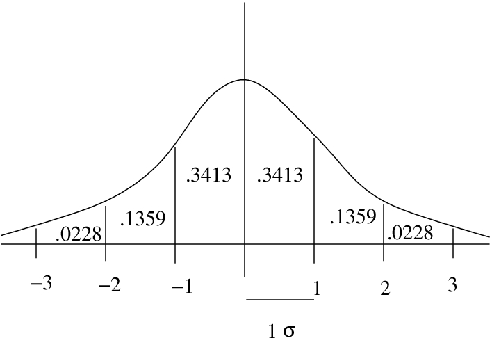Figure 5.4 : The units of $z$ in $P(z)$ are standard deviations. No matter what the measurement units of $x$ were before the $z$ -transformation, the units of $z$ are “standardized” to be standard deviation units. With SPSS you will learn how to standardize ( $z$ -transform) variables so that you can sensibly combine multiple dependent variables into one dependent variable for univariate statistical analysis. The areas, probabilities, associated with each increment in $\sigma$ are shown here.

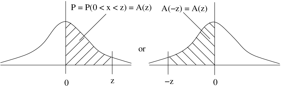
Let’s divide the types of areas we want to compute into cases, following Bluman^[4]. For all these cases we’ll use the notation $A(z)$ to represent the area we look up in the Standard Normal Distribution Table associated with $z$ .

Case 1 : Areas on one side of the mean. This is the case of finding an area between 0 (which corresponds to the mean before any $z$ -transformations) and a given $z$ . For this case we simply use the tabulated values, $P(0 \leq x \leq z)=A(z)$ , see Figure 5.5. This case also covers when $z$ is a negative number: $P(-z \leq x \leq 0)=A(z)$ .

Figure 5.5 : Case 1: Areas on one side of the mean.

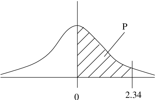
Example 5.1 : Find the probability that $z$ is between 0 and 2.34.

Solution : Look up $A(2.34)$ in the Standard Normal Distribution Table, see Figure 5.6. $P = P(0 < z < 2.34) = A(2.34) = 0.4904$ . (Note that it makes no difference whether we use $<$ or $\leq$ because the probability of a single value is 0. That’s why we need to use areas.)

Figure 5.6 : The situation for Example 5.1.

▢

Example 5.2 : Find the probability that $z$ is between -1.75 and 0.

Solution : $P(-1.75 < z < 0) = A(1.75) = 0.4599$ , see Figure 5.7.

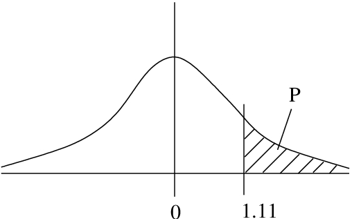
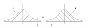
Figure 5.7 : The situation for Example 5.2.

▢

Case 2 : Tail areas. A tail area is the opposite of the area given in the Standard Normal Distribution Table on one half of the normal distribution, see Figure 5.8. The tail area after a given positive $z$ is $P = P(x > z) = 0.5 - A(z)$ or before a given negative value $-z$ is $P = P(x < -z) = 0.5 - A(z)$ .

Example 5.3 : What is the probability that $z > 1.11$ ?

Solution : $P(z > 1.11) = 0.5 - A(1.11) = 0.5 - 0.3665 = 0.1335$ , see Figure 5.9.

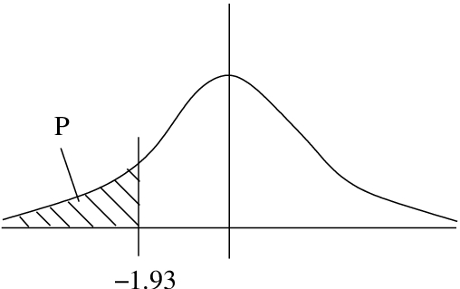
Figure 5.9 : The situation for Example 5.3.

▢

Example 5.4 : What is the probability that $z < -1.93$ ?

Solution : $P = P(z < -1.93) = 0.5 - A(1.93) = 0.5 - 0.4732 = 0.0268$ , see Figure 5.10.

Figure 5.10 : The situation for Example 5.2.

▢

Case 3 : An interval on one side of the mean. Recall that $\mu=0$ for the $z$ -distribution. So we are looking for the probabilities $P = P(z_{1} < x < z_{2})$ for an interval to the right of the mean or $P = P(-z_{2} < x <- z_{1})$ for an interval to the left of the mean. In either case $P = A(z_{2}) - A(z_{1})$ , see Figure 5.11.

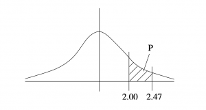
Figure 5.11: Case 3: An interval on one side of the mean.

Example 5.5 : What is the probability that $z$ is between 2.00 and 2.97?

Solution : $P(2.00 < z < 2.97) = A(2.47) - A(2.00) = 0.4932 - 0.4772 = 0.0160$ , see Figure 5.12.

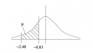
Figure 5.12: The situation for Example 5.5.

▢

Example 5.6 : What is the probability that $z$ is between -2.48 and -0.83?

Solution : $P(-2.48 < z < -0.83) = A(2.48) - A(0.83) = 4.934 - 0.2967 = 0.1967$ , see Figure 5.13.

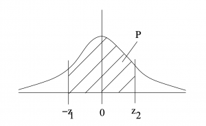
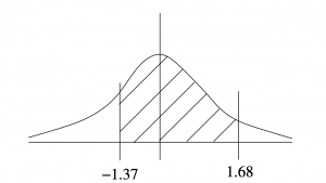
Figure 5.13: The situation of Example 5.6.

▢

Case 4 : An interval containing the mean. The situation is as shown in Figure 5.14 with the interval being between a negative and a positive number. In that case $P(-z_{1} < x < z_{2}) = A(z_{1}) + A(z_{2})$ .

Figure 5.14: Case 4: An interval containing the mean.

Example 5.7 : What is the probability that $z$ is between -1.37 and 1.68?

Solution : $P(-1.37 < z < 1.68) = A(1.37) + A(1.68) = 0.4147 + 0.4535 = 0.8682$ , see Figure 5.15.

Figure 5.15: The situation for Example 5.7.

▢

Cases 5 & 6 : Excluding tails. Case 5 is excluding the right tail, $P(x < z)$ . Case 6 is excluding the left tail, $P(x > -z)$ . See Figure 5.16. Case 5 is the situation which gives the percentile position of $z$ if you multiply the are by 100. More about percentiles in Chapter 6. In either case, $P = 0.5 + A(z)$ .

Figure 5.16: Left: Case 5. Right: Case 6.

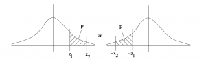
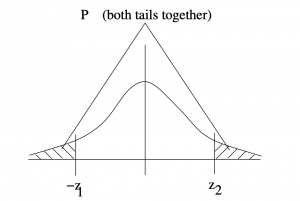
Case 7 : Two unequal tails. In this case we add the areas of the left and right tails, see FIgure 5.17. The special case where the tails have equal areas (i.e. when $z_{1} = z_{2}$ in the notation we have been using) is the case we will encounter for two-tail hypothesis testing. $P = P(x< -z_{1}) + P(x < z_{2}) = (0.5 - A(z_{1})) + (0.5 - A(z_{2}))$ .

Example 5.8 : Find the areas of the tails shown in Figure 5.18.

Solution :

$P(z < -3.01 \mbox{ or } z > 2.43)$
$= (0.5 - A(3.01)) + (0.5 - A(2.43))$
$= (0.5 - 0.4987) + (0.5 - 0.4925)$
$= 0.0013 + 0.0075$
$= 0.0088$ .

Figure 5.18: The situation for Example 5.8.

▢

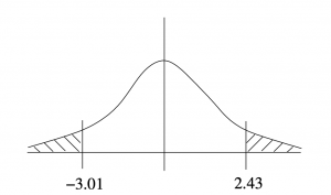
Using the Standard Normal Distribution Table backwards

Up until now we’ve used the Standard Normal Distribution Table directly. For a given $z$ , we look up the area $A(z)$ . Now we look at how to use it backwards: We have a number that represents the area between 0 and $z$ , what is $z$ ? Let’s illustrate this process with an example.

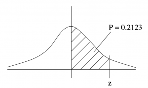
Example 5.9 : We are given an area $P=0.2123$ as shown in Figure 5.19. What is {z}?

Solution : Look in the Standard Normal Distribution Table for the closest value to the given $P$ . In this case 0.2123 corresponds exactly to $z = 0.56$ .

Figure 5.19: The situation for Example 5.9.

▢

Example 5.9 was artificial in that the given area appeared exactly in the Standard Normal Distribution Table. Usually it doesn’t. In that case pick the nearest area in the table to the given number and use the $z$ associated with the nearest area. This, of course, is an approximation. For those who know how, linear interpolation can be used to get a better approximation for $z$ .

The $z$ -transformation preserves areas

In a given situation of sampling a normal population, the mean and standard deviation of the population are not necessarily 0 and 1. We have just learned how to compute areas under a standard normal curve. How do we compute areas under an arbitrary normal curve? We use the $z$ -transformation. If we denote the original normal distribution by $P(x)$ and the $z$ -transformed distribution by $P(z)$ then areas under $P(x)$ will be transformed to areas under $P(z)$ that are the same. The $z$ -transformation preserves areas. So we can compute areas, or probabilities under $P(z)$ using the Standard Normal Distribution Table and instantly have the probabilities we need for the original $P(x)$ . Let’s follow an example.

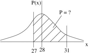
Example 5.10 : Suppose we know that the amount of garbage produced by households follows a normal distribution with a mean of $\mu = 28$ pounds/month and a standard deviation of $\sigma = 2$ pounds/month. What is the probability of selecting a household that produces between 27 and 31 pounds of trash/month?

Solution : First convert $x=27$ and $x=31$ to their $z$ -scores:

$z_{1} = z(27) = \frac{27-28}{2} = \frac{-1}{2} = -0.5$

$z_{2} = z(31) = \frac{31-28}{2} = \frac{3}{2} = 1.5$

Then, referring to Figure 5.20, we see that the probability is $P = A(0.5) + A(1.5) = 0.1915 + 0.4332 = 0.6247$ .

→ z-transform →

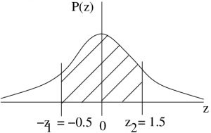
Figure 5.20 : The situation of Example 5.10. Left is the given population, $P(x)$ . On the right is the $z$ -transformed version of the population $P(z)$ . The value 27 is $z$ -transformed to -0.5 and 31 is $z$ -transformed to 1.5.

▢

In Example 5.10 we used the Standard Normal Distribution Table directly. You will also need to know how to solve problems in which you use this table backwards. The next example shows how that is done. For this kind of problem you will find the $z$ first and then you will need to find $x$ using the inverse $z$ -transformation :

$x = z \cdot \sigma + \mu.$

which is derived by solving the $z$ -transformation, $z = \frac{x-\mu}{\sigma}$ for $x$ .

Example 5.11 : In this example we work from given $P$ . To be a police person you need to be in the top 10\% on a test that has results that follow a normal distribution with an average of $\mu = 200$ and $\sigma = 20$ .

What score do you need to pass?

Solution : First, find the $z$ such that $P = P(y > z) = 0.10$ . That $P$ is a right tail area (Case 2), so we need $A(z) = 0.4$ , look at Figure 5.21 to see that. Then, going to the Standard Normal Distribution Table, look for 0.4 in the middle of the table then read off $z$ backwards. The closest area is 0.3997 which corresponds to $z = 1.28$ . Using the inverse $z$ -transformation, convert that $z$ to an $x$ :
to get

$x = 1.28 \times 20 + 200 = 25.60 + 200 = 225.60$

or, rounding, use $x = 226$ . There are frequently consequences to our calculations and in this case we want to make sure that we have a score that guarantees a pass. So we round the raw calculation up to ensure that.

← inverse z-transform ←

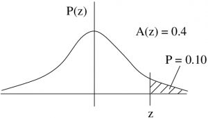
Figure 5.21 : The situation of Example 5.11

▢

**Whose shape is determined essentially by the shape of $y = e^{-{x}^{2}}$ . Plot $y = e^{-x}$ and think about the square preventing any negative values for the argument. ↵
** The number $e$ is the natural base implied by functions whose values match how fast it changes, i.e. the derivative of the function is the same as the function. ↵
** Of course, $\pi$ comes from circles: $\pi$ = circumference/diameter. ↵
Bluman AG, Elementary Statistics: A Step-by-Step Approach, numerous editions, McGraw-Hill Ryerson, circa 2005. ↵

License

Icon for the Creative Commons Attribution-NonCommercial-ShareAlike 4.0 International License

Introduction to Applied Statistics for Psychology Students Copyright © 2022 by Gordon E. Sarty is licensed under a Creative Commons Attribution-NonCommercial-ShareAlike 4.0 International License, except where otherwise noted.

5.3.1 Computing Areas (Probabilities) under the standard normal curve

License

Share This Book