
14. Correlation and Regression
14.5 Linear Regression
Linear regression gives us the best equation of a line through the scatter plot data in terms of least squares. Let’s begin with the equation of a line:
![\[ y = a + bx \]](https://openpress.usask.ca/app/uploads/quicklatex/quicklatex.com-ae090d17d1079208ae046cca3e21260a_l3.png "Rendered by QuickLaTeX.com")
where  is the intercept and
  is the slope.

The data, the collection of  points, rarely lie on a perfect straight line in a scatter plot. So we write
![\[ y^{\prime} = a + b x \]](https://openpress.usask.ca/app/uploads/quicklatex/quicklatex.com-37799dfd60164e46408e9d2190a1160a_l3.png "Rendered by QuickLaTeX.com")
as the equation of the best fit line. The quantity  is the predicted value of
  (predicted from the value of
  ) and is the measured value of . Now consider :

The difference between the measured and predicted value at data point  ,
,  , is the deviation. The quantity
![\[ d^{2}_{i} = (y_{i} - y^{\prime}_{i})^{2} = (y_{i} - (a + b x_{i}))^{2} \]](https://openpress.usask.ca/app/uploads/quicklatex/quicklatex.com-08af6db688b0db57c7e9045ff3cb7e66_l3.png "Rendered by QuickLaTeX.com")
is the squared deviation. The sum of the squared deviations is
![\[ E = \sum_{i=1}^{n} d_{i}^{2} = \sum_{i=1}^{n} (y_{i} - (a + b x_{i}))^{2} \]](https://openpress.usask.ca/app/uploads/quicklatex/quicklatex.com-7a19be5e930eb8184059e307311e383b_l3.png "Rendered by QuickLaTeX.com")
The least squares solution for and is the solution that minimizes  , the sum of squares, over all possible selections of and . Minimization problems are easily handled with differential calculus by solving the differential equations:
![\[ \frac{\partial E}{\partial a}=0 \;\;\;\;\; \mbox{and} \;\;\;\;\; \frac{\partial E}{\partial b}=0 \]](https://openpress.usask.ca/app/uploads/quicklatex/quicklatex.com-e99af988f3059de8e8fb31072b1073c6_l3.png "Rendered by QuickLaTeX.com")
The solution to those two differential equations is
![\[ a = \frac{(\sum y_{i})(\sum x_{i}^{2}) - (\sum x_{i})(\sum x_{i} y_{i})}{n(\sum x_{i}^{2}) - (\sum x_{i})^{2}} \]](https://openpress.usask.ca/app/uploads/quicklatex/quicklatex.com-db1a8fbc8784b06c1aad49cf0506ae45_l3.png "Rendered by QuickLaTeX.com")
and
![\[ b = \frac{n(\sum x_{i} y_{i}) - (\sum x_{i})(\sum y_{i})}{n(\sum x_{i}^{2}) - (\sum x_{i})^{2}} \]](https://openpress.usask.ca/app/uploads/quicklatex/quicklatex.com-def230a20776042b126a606e9c6c6005_l3.png "Rendered by QuickLaTeX.com")
Example 14.3 : Continue with the data from Example 14.1 and find the best fit line. The data again are:
| Subject | |
|
 |
 |
 |
| A | 6 | 82 | 492 | 36 | 6724 |
| B | 2 | 86 | 172 | 4 | 7396 |
| C | 15 | 43 | 645 | 225 | 1849 |
| D | 9 | 74 | 666 | 81 | 5476 |
| E | 12 | 58 | 696 | 144 | 3364 |
| F | 5 | 90 | 450 | 25 | 8100 |
| G | 8 | 78 | 624 | 64 | 6084 |
 |
 |
 |
 |
 |
 |
Using the sums of the columns, compute:

and

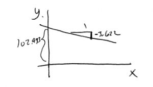
So

▢
14.5.1: Relationship between correlation and slope
The relationship is
![\[ r = \frac{b s_{x}}{s_{y}} \]](https://openpress.usask.ca/app/uploads/quicklatex/quicklatex.com-472a09bcf2057440a382ad0baaebd23d_l3.png "Rendered by QuickLaTeX.com")
where

are the standard deviations of the and datasets considered separately.
