13.1 Power

Gordon E. Sarty

13. Power

13.1 Power

Power is a concept that applies to all statistical testing. Here we will look at power quantitatively for the $z$ -test for means ( $t$ -test with large $n$ ). We will see explicitly in that case some principles that apply to other tests. These principles are: the bigger your sample size ( $n$ ), the higher the power; the larger $\alpha$ is, the more power there is^[1]; the larger the “effect size” is the more power there is. A final principle, that we can’t show by restricting ourselves to a $z$ -test, is that the simpler the statistical test, the more power it has — being clever doesn’t get you anywhere in statistics.

Let’s being by recalling the “confusion matrix” (here labelled a little differently than the one shown in Chapter 9 to emphasize the decision making). Note: The $\alpha$ , $\beta$ , etc. quantities are the probabilities that each conclusion will happen.

Reality

$H_{0}$

$H_{1}$

Conclusion of Test

$H_{1}$

Type I error
$\alpha$

Correct decision
$1-\beta$

$H_{0}$

Correct decision
$1-\alpha$

Type II error
$\beta$

Recall that $1 - \beta$ is the power, the probability of correctly rejecting $H_{0}$ . With the definition of $H_{1}$ as not $H_{0}$ , we cannot actually compute a power because this definition is too vague. The confusion matrix with $H_{0}$ and $H_{1}$ as given here is purely a conceptual device. To actually compute a power number we need to nail down a specific alternate hypothesis $H_{a}$ and compute $\beta$ for the more specific confusion matrix:

Reality

$H_{0}$

$H_{a}$

Conclusion of Test

$H_{a}$

Type I error
$\alpha$

Correct decision
$1-\beta$
(power)

$H_{0}$

Correct decision
$1-\alpha$

Type II error
$\beta$

We will define $H_{0}$ and $H_{a}$ be three parameters. The first is that we assume that the populations associated with $H_{0}$ and $H_{a}$ both have the same standard deviation $\sigma$ . Then, assuming that both populations are normal, $H_{0}$ is defined by its population mean $\mu_{0}$ (we used $k$ in Chapter 9) and $H_{a}$ is defined by its population mean $\mu_{a}$ .

We can define two flavors of power :

Predicted power. Based on a pre-defined alternate mean $\mu_{a}$ of interest and an estimate of $\sigma/\sqrt{n}$ . The population standard deviation $\sigma$ is frequently estimated from the sample standard deviation $s$ of a small pilot study.
Observed power. Based on the observed sample mean $\overline{x}$ which is then used as the alternate mean $\mu_{a}$ and sample standard deviation $s$ which is used for $\sigma$ .

The type II error rate $\beta$ (and power $1 - \beta$ ) is calculated by considering the populations associated with $H_{0}$ and $H_{1}$ :

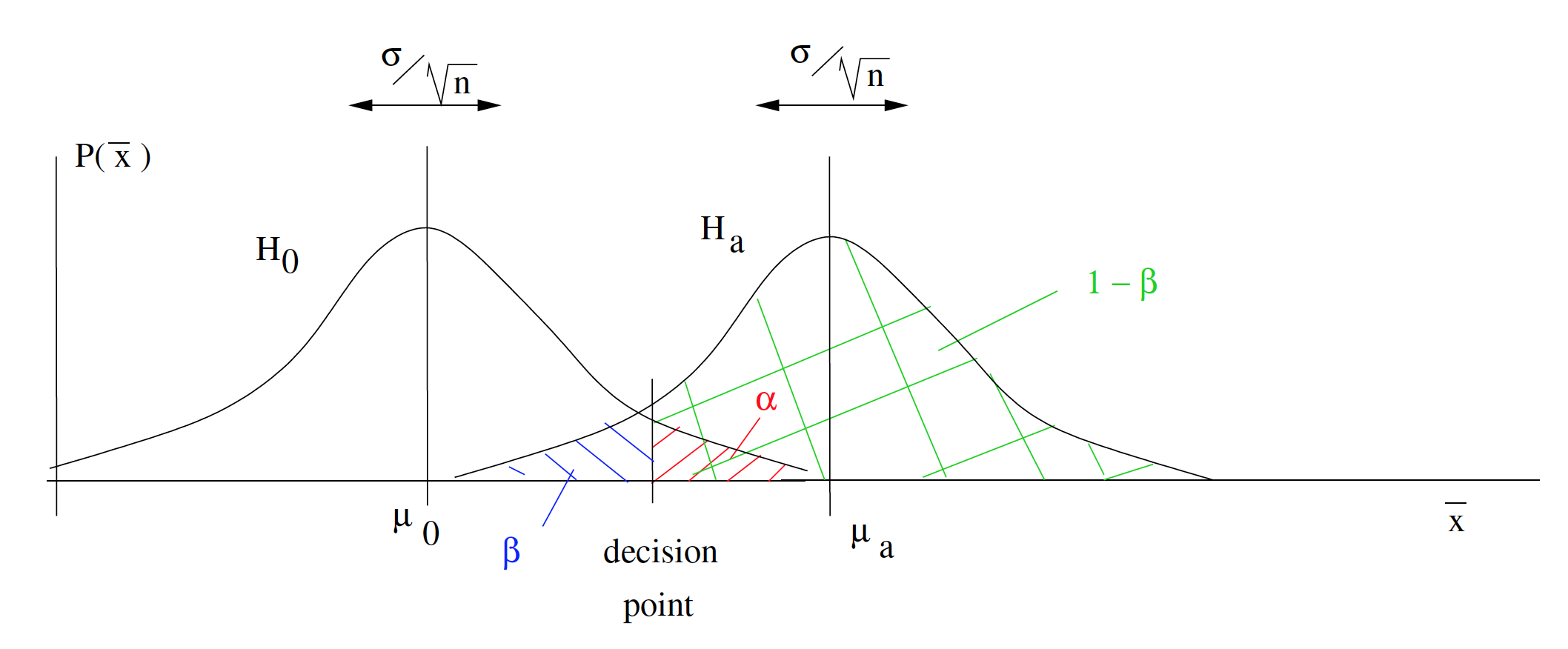
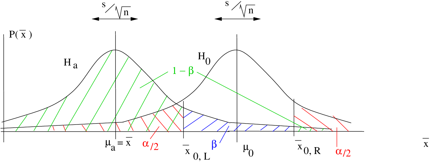
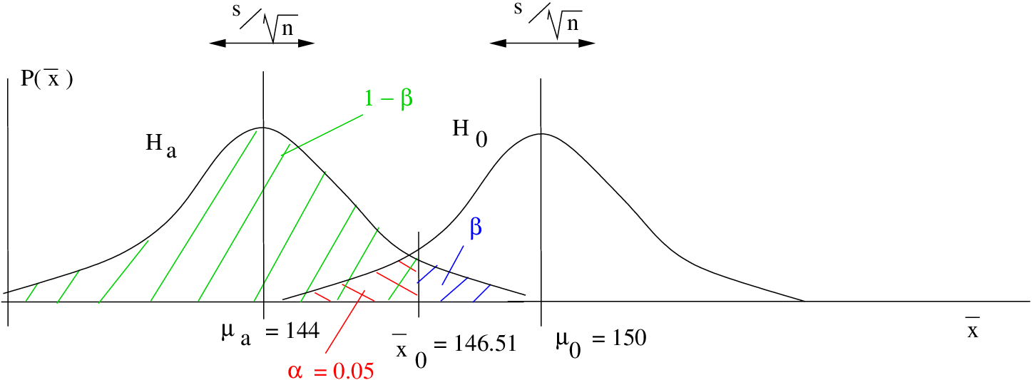
This picture follows directly from the Central Limit Theorem. Hypothesis testing is a decision process. In the picture above, which shows a one-tailed $z$ -test for means, you reject $H_{0}$ if $\overline{x}$ falls to the right of the decision point. The decision point is set by the value of $\alpha$ . Note that the alternate mean $\mu_{a}$ needs to be in the rejection region of $H_{0}$ for the picture to make sense. The value of $\beta$ (and hence the power $1 - \beta$ ) depends on the magnitude of the effect size^[2] $\mu_{a} - \mu_{0}$ . We can see that power will increase if the effect size that we are looking for in our experiment increases. This makes sense because larger differences should be easier to measure. Also note that if $n$ increases, as it would by replicating an experiment with a larger sample size, then the two distributions of sample means will get skinner and, for a given effect size, the power will increase. Again, this makes intuitive sense because more data is always better. We will illustrate these features in the numerical examples that follow.

For the purpose of learning the mechanics of statistical power we focus on observed power. With observed power we use the sample data for the power calculations; set $\mu_{a} = \overline{x}$ and $\sigma = s$ . Since $\mu_{a}$ needs to be in the rejection region of $H_{0}$ , observed power can only be computed when the conclusion of the hypothesis test is to reject $H_{0}$ . In real life if you reject $H_{0}$ you don’t care about what power the experiment had to reject $H_{0}$ . It’s a bit like calculating if you have enough gas to drive to Regina after you’ve arrived at Regina. In real life you will care about power only if you fail to reject $H_{0}$ because you will want to know the problem was that you tried to measure too small of an effect size or if a larger sample might lead to a decision to reject $H_{0}$ . In that case you will need to decide what effect size, or sample size, to use in computing a predicted power. You will use predicted power in your experiment design. If your experiment design has a predicted power of about 0.80 then you have a reasonable chance of rejecting the null hypothesis. If your research involves invasive intervention with people (needles, surgery, etc.) then you may need to present a power calculation to prove to an ethics committee that your experiment has a reasonable chance of finding what you think it will find.

In addition to $\mu_{a} = \overline{x}$ and $\sigma = s$ we need the value of the decision point $\overline{x}_{0}$ which is the inverse $z$ -transform of $z_{\alpha} = z_{\mbox{crit}}$ . We’ll consider three cases :

Case 1. Right tailed test:

$H_{0}: \mu \leq \mu_{0} \;\;\;\;\;\;\; H_{1}: \mu > \mu_{0}$

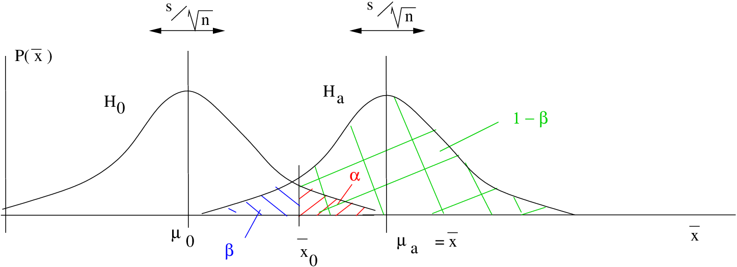
where, In this case

$\overline{x}_{0} = \mu_{0} + z_{\alpha} \left( \frac{s}{\sqrt{n}} \right)$

Case 2. Left tailed test:

$H_{0}: \mu \geq \mu_{0} \;\;\;\;\;\;\; H_{1}: \mu < \mu_{0}$

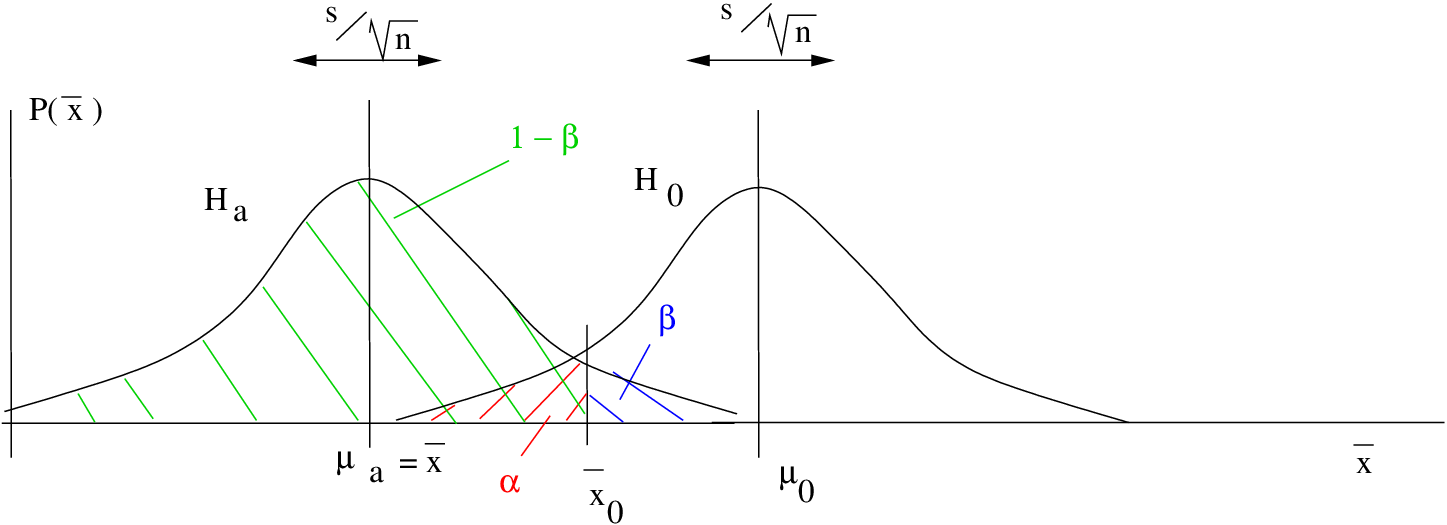
where, In this case

$\overline{x}_{0} = \mu_{0} - z_{\alpha} \left( \frac{s}{\sqrt{n}} \right)$

Case 3. Two-tailed test:

$H_{0}: \mu = \mu_{0} \;\;\;\;\;\;\; H_{1}: \mu \neq \mu_{0}$

(a) $\overline{x}$ in the right tail :

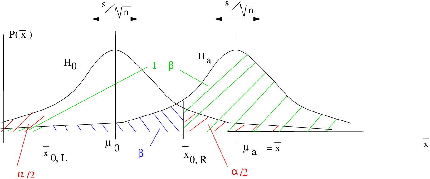
(b) $\overline{x}$ in the left tail:

where, in both cases:

$\begin{eqnarray*} \overline{x}_{0,L} & = & \mu_{0} - z_{\alpha/2} \left( \frac{s}{\sqrt{n}} \right) \\ \overline{x}_{0,R} & = & \mu_{0} + z_{\alpha/2} \left( \frac{s}{\sqrt{n}} \right) \end{eqnarray*}$

In both two-tailed cases, notice the small piece of $1 - \beta$ area on the side of the $H_{a}$ distribution on the opposite side from $\overline{x}$ . It turns out that the area of that small part is so incredibly small that we can take it to be zero. This will be obvious she we work through the examples. So the upshot is that going from a one-tailed test to a two-tailed test effectively decreases $\alpha$ to $\alpha/2$ which increases $\beta$ and decreases the power $1 - \beta$ . One-tailed tests have more power than two-tailed tests for the same $\alpha$ .

Example 13.1 Right tailed test.

Given :

$H_{0}: \mu \leq 150, H_{1} > 150$

$n = 50$ , $\alpha = 0.05$ , $s = 15$ , $\overline{x} = \mu_{a} = 155$

Find the observed power.

Step 1 : Look up $z_{\alpha} = z_{0.05}$ in the t Distribution Table for a one-tailed test: $z_{\alpha} = 1.645$ .

Step 2 : Compute :

$\begin{eqnarray*} \overline{x}_{0} & = & \mu_{0} + z_{\alpha} \left( \frac{s}{\sqrt{n}} \right) \\ & = & 150 + (1.645) \left( \frac{15}{\sqrt{50}} \right) \\ & = & 153.49 \end{eqnarray*}$

Step 3 : Draw picture :

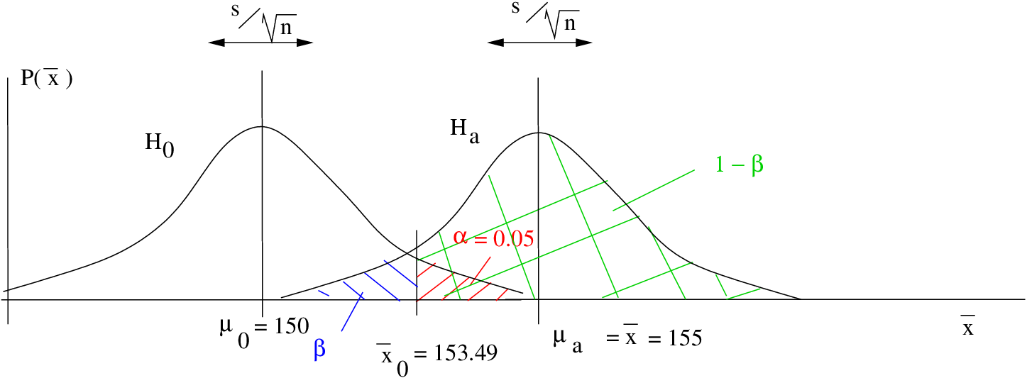
Step 4 : Compute the $z$ -transform of $\overline{x}_{0}$ relative to $H_{a}$ :

$\begin{eqnarray*} z_{a} & = & \frac{\overline{x}_{0} - \mu_{a}}{\left( s / \sqrt{n} \right)} \\ & = & \frac{153.49 - 155}{\left( 15 / \sqrt{50} \right)} \\ & = & -0.71 \end{eqnarray*}$

Step 5 : Look up the area $A(-z_{a})$ in the Standard Normal Distribution Table. That area will be $0.5 - \beta$ : $0.5 - \beta = 0.2611$ , so $\beta = 0.5 - 0.2611 = 0.2389$ and power = $1 - \beta = 1 - 0.2389 =$ 0.7611.

▢

Example 13.2 : Another right tailed test with the data the same as in Example 13.1 but with a smaller $\alpha$ . This example shows how reducing $\alpha$ will reduce the power. With reduced power, it is harder to reject $H_{0}$ .

Given :

$H_{0}: \mu \leq 150, H_{1} > 150$

$n = 50$ , $\alpha = 0.01$ , $s = 15$ , $\overline{x} = \mu_{a} = 155$

Find the observed power.

Step 1 : Look up $z_{\alpha} = z_{0.01}$ in t Distribution Table for a one-tailed test: $z_{\alpha} = 2.326$ .

Step 2 : Compute :

$\begin{eqnarray*} \overline{x}_{0} & = & \mu_{0} + z_{\alpha} \left( \frac{s}{\sqrt{n}} \right) \\ & = & 150 + (2.326) \left( \frac{15}{\sqrt{50}} \right) \\ & = & 154.93 \end{eqnarray*}$

Step 3 : Draw picture :

Step 4 : Compute the $z$ -transform of $\overline{x}_{0}$ relative to $H_{a}$ :

$\begin{eqnarray*} z_{a} & = & \frac{\overline{x}_{0} - \mu_{a}}{\left( s / \sqrt{n} \right)} \\ & = & \frac{154.93 - 155}{\left( 15 / \sqrt{50} \right)} \\ & = & -0.03 \end{eqnarray*}$

Step 5 : Look up the area $A(0.03)$ in the Standard Normal Distribution Table. That area will be $A(0.03) = 0.0120$ . So $\beta = 0.5 - 0.0120 = 0.4880$ and power = $1 - \beta =$ 0.5120 which is smaller than the power found in Example 13.1.

▢

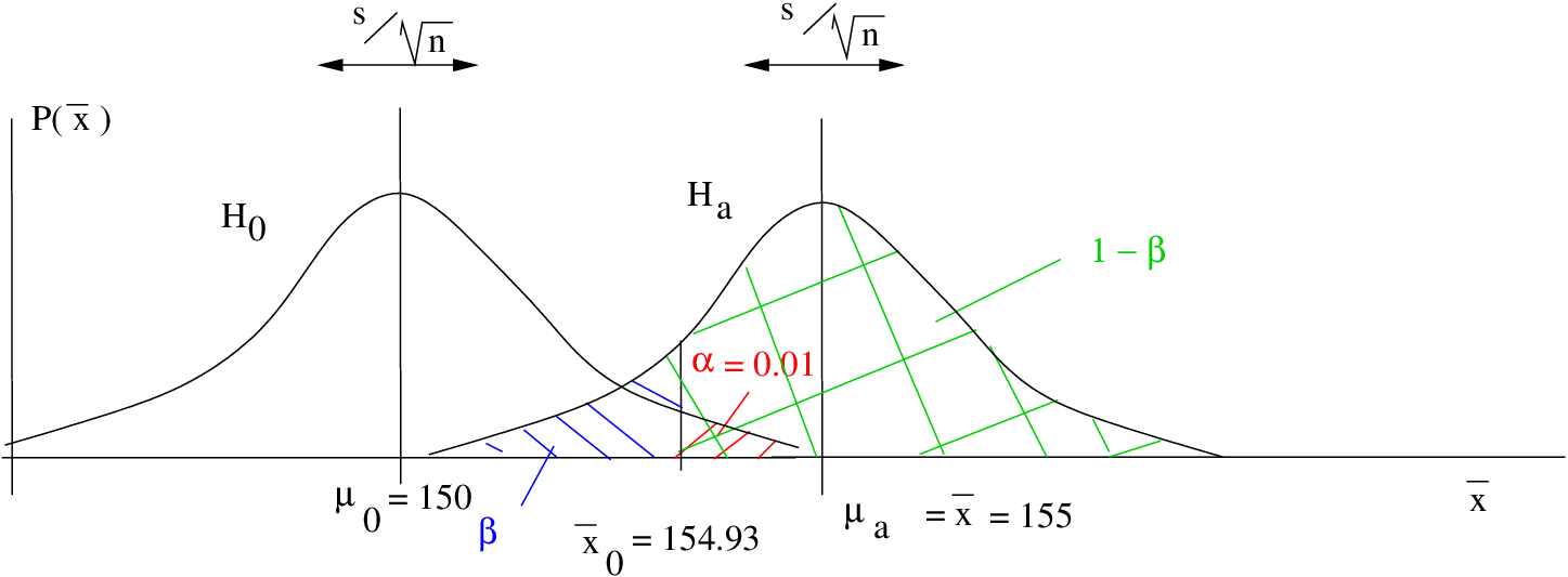
Example 13.3 : Another right tailed test with the data the same as in Example 13.2 but with larger $n$ . This example shows how increasing the sample size increases the power. This makes sense because more data is always better.

Given :

$H_{0}: \mu \leq 150, H_{1} > 150$

$n = 150$ , $\alpha = 0.01$ , $s = 15$ , $\overline{x} = \mu_{a} = 155$

Find the observed power.

Step 1 : Look up $z_{\alpha} = z_{0.01}$ in t Distribution Table for a one-tailed test: $z_{\alpha} = 2.326$ .

Step 2 : Compute :

$\begin{eqnarray*} \overline{x}_{0} & = & \mu_{0} + z_{\alpha} \left( \frac{s}{\sqrt{n}} \right) \\ & = & 150 + (2.326) \left( \frac{15}{\sqrt{150}} \right) \\ & = & 152.85 \end{eqnarray*}$

Step 3 : Draw picture :

Step 4 : Compute the $z$ -transform of $\overline{x}_{0}$ relative to $H_{a}$ :

$\begin{eqnarray*} z_{a} & = & \frac{\overline{x}_{0} - \mu_{a}}{\left( s / \sqrt{n} \right)} \\ & = & \frac{152.85 - 155}{\left( 15 / \sqrt{150} \right)} \\ & = & -1.76 \end{eqnarray*}$

Step 5 : Look up the area $A(0.03)$ in the Standard Normal Distribution Table. That area will be $A(0.03) = 0.4808$ . So $\beta = 0.5 - 0.4808 = 0.0392$ and power = $1 - \beta =$ 0.9608 which is larger than the power found in Example 13.2.

▢

Example 13.4 : Another right tailed test with the data the same as in Example 13.3 but with a smaller value for $\overline{x} = \mu_{a}$ which leads to a smaller effect size. This example shows how decreasing the effect size decreases the power. This makes sense because it is harder to detect a smaller signal.

Given :

$H_{0}: \mu \leq 150, H_{1} > 150$

$n = 150$ , $\alpha = 0.01$ , $s = 15$ , $\overline{x} = \mu_{a} = 153$

Find the observed power.

Step 1 : Look up $z_{\alpha} = z_{0.01}$ in the t Distribution Table for a one-tailed test: $z_{\alpha} = 2.326$ .

Step 2 : Compute :

$\begin{eqnarray*} \overline{x}_{0} & = & \mu_{0} + z_{\alpha} \left( \frac{s}{\sqrt{n}} \right) \\ & = & 150 + (2.326) \left( \frac{15}{\sqrt{150}} \right) \\ & = & 152.85 \end{eqnarray*}$

Step 3 : Draw picture :

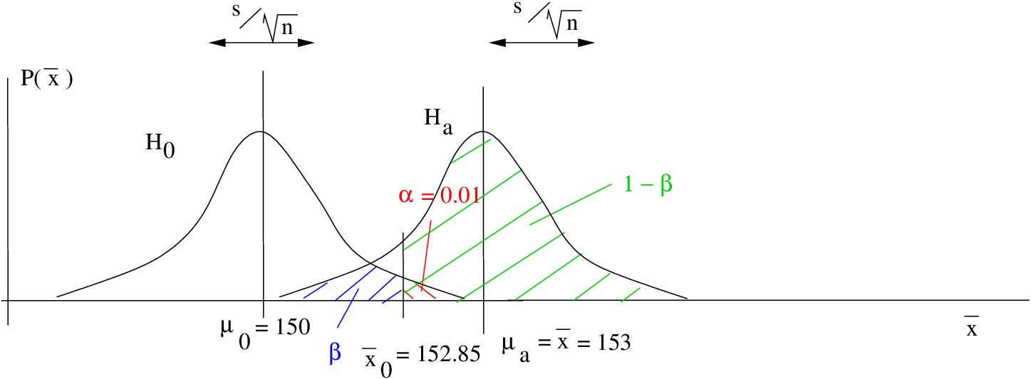
Step 4 : Compute the $z$ -transform of $\overline{x}_{0}$ relative to $H_{a}$ :

$\begin{eqnarray*} z_{a} & = & \frac{\overline{x}_{0} - \mu_{a}}{\left( s / \sqrt{n} \right)} \\ & = & \frac{152.85 - 153}{\left( 15 / \sqrt{150} \right)} \\ & = & -0.122 \end{eqnarray*}$

Step 5 : Look up the area $A(0.12)$ in the Standard Normal Distribution Table. That area will be $A(0.12) = 0.0478$ . So $\beta = 0.5 - 0.0478 = 0.4522$ and power = $1 - \beta =$ 0.5478 which is smaller than the power found in Example 13.3.

▢

Example 13.5 : Left tailed test.

Given :

$H_{0}: \mu \geq 150$ , $H_{1} < 150$

$n = 50$ , $\alpha = 0.05$ , $s = 15$ , $\overline{x} = \mu_{a} = 144$

Find the observed power.

Step 1 : Look up $z_{\alpha} = z_{0.05}$ in the t Distribution Table for a one-tailed test: $z_{0.05} = 1.645$ .

Step 2 : Compute :

$\begin{eqnarray*} \overline{x}_{0} & = & \mu_{0} - z_{\alpha} \left( \frac{s}{\sqrt{n}} \right) \\ & = & 150 - (1.645) \left( \frac{15}{\sqrt{50}} \right) \\ & = & 146.51 \end{eqnarray*}$

Step 3 : Draw picture :

Step 4 : Compute the $z$ -transform of $\overline{x}_{0}$ relative to $H_{a}$ :

$\begin{eqnarray*} z_{a} & = & \frac{\overline{x}_{0} - \mu_{a}}{\left( s / \sqrt{n} \right)} \\ & = & \frac{146.51 - 144}{\left( 15 / \sqrt{50} \right)} \\ & = & 1.18 \end{eqnarray*}$

Step 5 : Look up the area $A(1.18)$ in the Standard Normal Distribution Table. That area will be $A(1.18) = 0.3810$ . So $\beta = 0.5 - 0.3810 = 0.1190$ and power = $1 - \beta =$ 0.8810.

▢

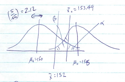
Example 13.6 : Two tailed $z$ -test with data the same as Example 13.5.

Given :

$H_{0}: \mu = 150$ , $H_{1} \neq150$

$n = 50$ , $\alpha = 0.05$ , $s = 15$ , $\overline{x} = \mu_{a} = 144$

Find the observed power.

Step 1 : Look up $z_{\alpha/2} = z_{0.025}$ in the t Distribution Table for a one-tailed test: $z_{0.025} = 1.960$ .

Step 2 : Compute:

$\begin{eqnarray*} \overline{x}_{0,L} & = & \mu_{0} - z_{\alpha/2} \left( \frac{s}{\sqrt{n}} \right) \\ & = & 150 - (1.960) \left( \frac{15}{\sqrt{50}} \right) \\ & = & 145.84 \end{eqnarray*}$

and

$\begin{eqnarray*} \overline{x}_{0,R} & = & \mu_{0} + z_{\alpha/2} \left( \frac{s}{\sqrt{n}} \right) \\ & = & 150 + (1.960) \left( \frac{15}{\sqrt{50}} \right) \\ & = & 154.16 \end{eqnarray*}$

Step 3 : Draw picture :

Step 4 : Compute the $z$ -transform of $\overline{x}_{0,L}$ and $\overline{x}_{0,R}$ relative to $H_{a}$ :

$\begin{eqnarray*} z_{a,L} & = & \frac{\overline{x}_{0,L} - \mu_{a}}{\left( s / \sqrt{n} \right)} \\ & = & \frac{145.84 - 144}{\left( 15 / \sqrt{50} \right)} \\ & = & 0.87 \end{eqnarray*}$

and

$\begin{eqnarray*} z_{a,R} & = & \frac{\overline{x}_{0,R} - \mu_{a}}{\left( s / \sqrt{n} \right)} \\ & = & \frac{154.16 - 144}{\left( 15 / \sqrt{50} \right)} \\ & = & 4.79 \end{eqnarray*}$

Step 5 : The two values, $z_{a,L}$ and $z_{a,R}$ appear on the $z$ -distribution as :

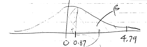
So using the areas $A(z)$ from the Standard Normal Distribution Table we find

$\beta = A(4.79) - A(0.87) = 0.5 - 0.3078 = 0.1922$

Notice that $z=4.79$ is way the heck out there, it is higher than any $z$ given in the Standard Normal Distribution Table. So $A(7.79)$ is essentially 0.5; the tail area past $z=4.79$ is essentially zero. So the effect of going to from a one-tail to a two-tail test is only felt by the size of the $H_{0}$ critical region on the side where the test statistic ( $\overline{x}$ here) is, which is half the size of the critical region in a one-tail test for a fixed $\alpha$ . In this case, then, the power = $1 - \beta =$ 0.8078 which is smaller than the value found in Example 13.5.

▢

Using observed power

As mentioned earlier, almost no one is interested in observed power because we must reject $H_{0}$ to compute it. People are interested in $\beta$ and power only when you report a failure to reject $H_{0}$ .

Suppose in the situation of Example 13.1 we wanted to find evidence that $\mu_{a} = 155$ but measured $\overline{x} = 152$ (fail to reject $H_{0}$ ). Then, with our given information of

$H_{0}: \mu \leq 150$ , $H_{1} > 150$

$n = 50$ , $\alpha = 0.05$ , $s = 15$ , $\overline{x} = 152$ and $\mu_{a} = 155$

we have

Based on the calculation we did in Example 13.1 we would report that we had a power of 0.7611 to detect an effect of $\mu_{a} = 155$ but with $\overline{x} = 152$ we were unable to detect $\mu_{a}$ .

And a corollary of this will be that one-tailed tests are more powerful than two-tailed tests. ↵
Effect size as defined in the Green and Salkind SPSS book would be $\mu_{a} - \mu_{0}/\sigma$ . But that quantity is not useful here, so we define effect size as the difference of the means for the purpose of this discussion on power. Reference: Green SB, Salkind NJ. Using SPSS for Windows and Macintosh: Analyzing and Understanding Data, new edition pretty much every year, Pearson, Toronto, circa 2005. ↵

License

Icon for the Creative Commons Attribution-NonCommercial-ShareAlike 4.0 International License

Introduction to Applied Statistics for Psychology Students Copyright © 2022 by Gordon E. Sarty is licensed under a Creative Commons Attribution-NonCommercial-ShareAlike 4.0 International License, except where otherwise noted.

Using observed power

License

Share This Book