
8. Confidence Intervals
8.3 The t-Distributions
As a broad introduction, the  -distributions are family of distributions that give different approximations to the
  -distribution as shown in Figure 8.5.
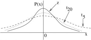 -distributions are a family of distributions, labeled here by their degrees of freedom
  as in
as in  .
.As the degrees of freedom, , increases, become closer to ,  . In practice, as reflected in the t Distribution Table,
  is very very close to .
The -distributions arise as a corollary to the central limit theorem; they give the distribution of sample means when knowledge of the population  is replaced by using the sample mean
  . When we encounter the
  distribution later, we will give a more exact mathematical specification of the -distributions.
Similar, to the -distribution case, the  confidence interval for the mean
  for small
  samples is given by
![\[ \bar{x} - E < \mu < \bar{x} + E\]](https://openpress.usask.ca/app/uploads/quicklatex/quicklatex.com-237c1639f5c8a6c0bbd2fc90ff3eb73b_l3.png "Rendered by QuickLaTeX.com")
where, now
![\[E = t_{\nu,\cal{C}} \left( \frac{s}{\sqrt{n}} \right).\]](https://openpress.usask.ca/app/uploads/quicklatex/quicklatex.com-9f1b81fdcac4355e61f401c02f38bca6_l3.png "Rendered by QuickLaTeX.com")
With this new formula for  we have replaced with in comparison with the formula we used in Section 8.1: Confidence Intervals using the z-distribution and, of course, replaced
  with
with  . Some books use
  like the of Section 8.1. We use because we’ll look up its value in the t Distribution Table in the column for confidence intervals (just like we did with ) and with the degrees of freedom specifying the row. The formula for the degrees of freedom in this case is :
![\[\nu = n - 1.\]](https://openpress.usask.ca/app/uploads/quicklatex/quicklatex.com-97834d804f01820a52c2711acfbe7b95_l3.png "Rendered by QuickLaTeX.com")
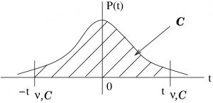
The specify a probability as shown in Figure 8.6. As before, the inverse -transform, in the form  from the -distribution on the left of Figure 8.6 to the distribution on the right of Figure 8.6 leads to our confidence interval formula for small means. And as before we should justify using that transform from a Bayesian perspective.
 → inverse -transform →
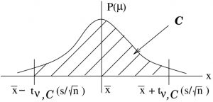
Figure 8.6 : Derivation of confidence intervals for means of small samples.
Example 8.2 : Given the following data:
![\[5460 \hspace{.15in} 5900 \hspace{.15in} 6090 \hspace{.15in} 6310 \hspace{.15in} 7160 \hspace{.15in} 8440 \hspace{.15in} 9930\]](https://openpress.usask.ca/app/uploads/quicklatex/quicklatex.com-0fd6658dbfefce6d589ffc0468fdf032_l3.png "Rendered by QuickLaTeX.com")
find the 99% confidence interval for the mean.
Solution : First count  and then, with your stats calculator compute
![\[ \bar{x} = 7041.4 \hspace{.15in} \text{and} \hspace{.15in} s = 1610.3. \]](https://openpress.usask.ca/app/uploads/quicklatex/quicklatex.com-2ba4fc2ef760b58c20e87347708722a9_l3.png "Rendered by QuickLaTeX.com")
Using the t Distribution Table with  in the 99% confidence interval column, find
![\[ t_{n-1, {\cal{C}}} = t_{6,99\%} = 3.707. \]](https://openpress.usask.ca/app/uploads/quicklatex/quicklatex.com-91b738496dbdc3cdc89212eb81d60869_l3.png "Rendered by QuickLaTeX.com")
With these numbers, compute
![\[ E = t_{n-1,{\cal{C}}} \left( \frac{s}{\sqrt{n}} \right) = 3.707 \left( \frac{1610.3}{\sqrt{7}} \right) = 2256.2 \]](https://openpress.usask.ca/app/uploads/quicklatex/quicklatex.com-8374dd093f70abb69b006bcb091be7d2_l3.png "Rendered by QuickLaTeX.com")
so

is the 99 confidence interval for .
▢
