10.2 Confidence Interval for Difference of Means (Large Samples)

Gordon E. Sarty

10. Comparing Two Population Means

10.2 Confidence Interval for Difference of Means (Large Samples)

Swapping the roles of sample and population in the sampling theory, we have the confidence interval corresponding to the hypothesis test of Section 10.1

$(\bar{x}_1 - \bar{x}_2) - E < (\mu_1 - \mu_2) < (\bar{x}_1 - \bar{x}_2) + E$

where

$E = z_{\cal C}\sqrt{\frac{s^2_1}{n_1} + \frac{s^2_2}{n_2}}$

Example 10.2 : Find the 95 $\%$ confidence interval for the difference between the means for the data of Example 10.1.

Solution : First, recall our data :

$\bar{x}_1 = 88.42$ , $s_1 = 5.62$ , $n_1 = 50$

$\bar{x}_2 = 80.61$ . $s_2 = 4.83$ , $n_2 = 50$

From the t Distribution Table, look up the $z$ for the 95 $\%$ confidence interval: $z_{95\%} = 1.960$ . Then compute:

$\bar{x}_1 - \bar{x}_2 = 88.42 - 80.61 = 7.81$

and

$\begin{eqnarray*} E & = & z_{95\%}\sqrt{\frac{s^2_1}{n_1} + \frac{s^2_2}{n_2}} \\ & = & 1.960\sqrt{\frac{5.62^2}{50} + \frac{4.83^2}{50}} \\ & = & 2.05 \end{eqnarray*}$

so

$7.81 - 2.05 < (\mu_1 - \mu_2) < 7.81 + 2.05$

or

$5.76 < (\mu_1 - \mu_2) < 9.83$

with 95 $\%$ confidence. Notice that it is also correct to write $\mu_{1} - \mu_{2} = 7.81 \pm 2.05$ with 95 $\%$ confidence.

▢

This is a good point to make an important observation. A two-tailed hypothesis test at a given $\alpha$ is complementary to a confidence interval of ${\cal{C}} = 1 - \alpha$ in the sense that if 0 is in the confidence interval then the complementary hypothesis test will not reject $H_{0}$ .

Let’s illustrate this principle with a one-sample $t$ -test under $H_{0}: \mu = 0$ . (We need $k=0$ for this principle to work.) Look at the two possible outcomes :

Case 1 : 0 in the confidence interval, fail to reject $H_{0}$ . In the hypothesis test you would find :

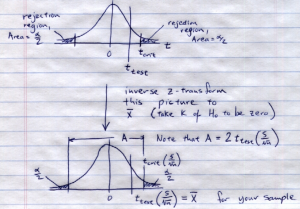
In the confidence interval calculation you would find:

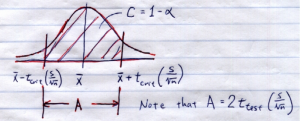
Putting the two pictures together gives:

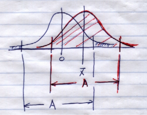
See, $0$ is in the confidence interval if ¯ $\bar{x}$ is not in the rejection region. The red distribution that defines the confidence interval is just the blue (identical) distribution slid over from $0$ to $\bar{x}$ . The distance $A$ is the same because ${\cal{C}} = 1 - \alpha$ .

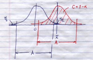
Case 2 : 0 not in the confidence interval, reject $H_{0}$ . In this case the combined picture looks like:

Before we can consider the independent sample $t$ -test, we need a tool for checking what the variances of the populations are. The formula for the $t$ test statistic will depend on whether the two variances are the same or not. So let’s take a look at comparing population variances.

License

Icon for the Creative Commons Attribution-NonCommercial-ShareAlike 4.0 International License

Introduction to Applied Statistics for Psychology Students Copyright © 2022 by Gordon E. Sarty is licensed under a Creative Commons Attribution-NonCommercial-ShareAlike 4.0 International License, except where otherwise noted.

License

Share This Book