3.1 Central Tendency: Mean, Median, Mode

Gordon E. Sarty

3. Descriptive Statistics: Central Tendency and Dispersion

3.1 Central Tendency: Mean, Median, Mode

Mean, median and mode are measures of the central tendency of the data. That is, as data are collected while sampling from a population, there values will tend to cluster around these measures. Let’s define them one by one.

3.1.1 Mean

The mean is the average of the data. We distinguish between a sample mean and a population mean with the following symbols :

$\bar{x} = sample\hspace{.1cm}mean$

$\mu = population\hspace{.1cm}mean$

The formula for a sample mean is :

$\bar{x} = \frac{ \sum_{i=1}^{n} x_{i} }{n}$

where $n$ is the number of data points in the sample, the sample size. For a population, the formula is

$\mu = \frac{ \sum_{i=1}^{N} x_{i} }{N}$

where $N$ is the size of the population.

Example 3.1 : Find the mean of the following data set :

84	12	27	15	40	18	33	33	14	4
$x_{1}$	$x_{2}$	$x_{3}$	$x_{4}$	$x_{5}$	$x_{6}$	$x_{7}$	$x_{8}$	$x_{9}$	$x_{10}$

To illustrate how the indexed symbols that represent the data in the formula work, they have been written below the data values. To get in the habit, let’s organize our data as a table. We will need to do that for more complicated formulae and also that’s how you need to enter data into SPSS, as a column of numbers :

$x$	label
84	$x_{1}$
12	$x_{2}$
27	$x_{3}$
15	$x_{4}$
40	$x_{5}$
18	$x_{6}$
33	$x_{7}$
33	$x_{8}$
14	$x_{9}$
4	$x_{10}$
Total = 280

Since $n = 10$ we have $\bar{x} = \frac{\sum x_{i}}{n} = \frac{280}{10} = 28$ .

☐

Mean for grouped data : If you have a frequency table for a dataset but not the actual data, you can still compute the (approximate) mean of the dataset. This somewhat artificial situation for datasets will be a fundamental situation when we consider probability distributions. The formula for the mean of grouped data is

(3.1) $\begin{equation*} \bar{x} = \frac{ \sum_{i=1}^{G} f_i x_{m_{i}}}{n}\ \end{equation*}$

where $f_{i}$ is the frequency of group $i$ , $x_{m_{i}}$ is the class center of group $i$ and $n$ is the number of data points in the original dataset. Recall that $n = \sum f_{i}$ so we can write this formula as

$\bar{x} = \frac{ \sum_{i=1}^{G} f_i x_{m_{i}}}{\sum_{i=1}^{G} f_{i}}$

which is a form that more closely matches with a generic weighted mean formula; the formula for the mean of grouped data is a special case of a more general weighted mean that we will look at next. The class center is literally the center of the class — the next example shows how to find it.

Example 3.2 : Find the mean of the dataset summarized in the following frequency table.

Class	Class Boundaries	Frequency, $f_{i}$	Midpoint, $x_{m_{i}}$	$f_{i}x_{m_{i}}$
1	5.5 – 10.5	1	8	8
2	10.5 – 15.5	2	13	26
3	15.5 – 20.5	3	18	54
4	20.5 – 25.5	5	23	115
5	25.5 – 30.5	4	28	112
6	30.5 – 35.5	3	33	99
7	35.5 – 40.5	2	38	76
sums		n= $\sum f_{i}$ = 20		$\sum f_{i}x_{m_{i}}$ = 490

Solution : The first step is to write down the formula to cue you to what quantities you need to compute :

$\bar{x} = \frac{\sum_{i} f_{i} x_{m_{i}}}{n}$

We need the sum in the numerator and the value for $n$ in the denominator. Get the numbers from the sums of the columns as shown in the frequency table :

$\bar{x} = \frac{\sum_{i} f_i x_{m_{i}}}{n} = \frac{490}{20} = 24.5$

☐

Note that the grouped data formula gives an approximation of the mean of the original dataset in the following way. The exact mean is given by

$\bar{x} = \frac{\sum_{i=1}^{n} x_{i}}{n} = \frac{\sum_{j=1}^{G} (\sum_{k=1}^{f_{i}} x_{k} ) }{n}.$

So the approximation is that

$\sum_{k=1}^{f_{i}} x_{k} = f_{i} x_{m_{i}}$

which would be exact only if all $x_{k}$ in group $i$ were equal to the class center $x_{m_{i}}$ .

Generic Weighted Mean : The general formula for weighted mean is

(3.2) $\begin{equation*} \bar{x} = \frac{\sum_{i=1}^{n} w_{i} x_{i}}{\sum_{i=1}^{n} w_{i}} \end{equation*}$

where $w_{i}$ is the weight for data point $i$ . Weights can be assigned to data points for a variety of reasons. In the formula for grouped data, as a weighted mean, treats the class centers as data points and the group frequencies as weights. The next example weights grades.

Example 3.3 : In this example grades are weighted by credit units. The weights are as given in the table :

Course	Credit Units, $w_{i}$	Grade, $x_{i}$	$w_{i}x_{i}$
English	3	80	240
Psych	3	75	225
Biology	4	60	240
PhysEd	2	82	164
	$\sum w_{i}$ = 12	$\sum x_{i}$ = 297	$\sum w_{i}x_{i}$ = 869

The formula for weighted mean is

$\bar{x} = \frac{\sum w_i x_i}{\sum w_i}$

so we need two sums. The double bars in the table above separate given data from columns added for calculation purposes. We will be using this convention with the double bars in other procedures to come. Using the sums for the table we get

$\bar{x} = \frac{\sum w_i x_i}{\sum w_i} = \frac{869}{12} = 72.4$

Note, that the unweighted mean for these data is

$\bar{x} = \frac{\sum x_i}{n} = \frac{297}{4} = 74.3$

which is, of course, different from the weighted sum.

☐

3.1.2 Median

The symbol we use for median is MD and it is the midpoint of the data set with the data put in order. We illustrate this with a couple of examples :

If there are an odd number of data points, MD is the middle number.

Given data in order: 180 186 191 201 209 219 220

$\uparrow$

$MD = 201$

If there are an even number of data points, MD is the average of the two middle points :

Given data in order: 656 684 702 764 856 1132 1133 1303

$\uparrow$ $\uparrow$

$MD = \frac{764 + 856}{2} = 810$

In these examples, the tedious work of putting the data in order from smallest to largest was done for us. With a random bunch of numbers, the work of finding the median is mostly putting the data in order.

3.1.3 Mode

In a given dataset the mode is the data value that occurs the most. Note that :

it may be there is no mode.
there may be more than one mode.

Example 3.4 : In the dataset

$\underline{8}$ , 9, 9, 14, $\underline{8}$ , $\underline{8}$ , 10, 7, 6, 9, 7, $\underline{8}$ , 10, 14, 11, $\underline{8}$ , 14, 11

8 occurs 5 times, more than any other number. So the mode is 8.

☐

Example 3.5 : The dataset

110, 731, 1031, 84, 20, 118, 1162, 1977, 103, 72

has no mode. Do not say that the mode is zero. Zero is not in the dataset.

☐

Example 3.6 : The dataset

15, $\underline{18, 18, 18,}$ 20, 22, $\underline{24, 24, 24,}$ 26, 26

has two modes: 18 and 24. This data set is bimodal.

The concept of mode really makes more sense for frequency table/histogram data.

☐

Example 3.7 : The mode of the following frequency table data is the class with the highest frequency.

Class	Class Boundaries	Freq
1	5.5 – 10.5	1
2	10.5 – 15.5	2
3	15.5 – 20.5	3
4	20.5 – 25.5	5 (Modal Class)
5	25.5 – 30.5	4
6	30.5 – 35.5	3
7	35.5 – 40.5	2

☐

3.1.4 Midrange

The midrange, which we’ll denote symbolically by MR, is defined simply by

$\mbox{MR} = \frac{H+L}{2}$

where $H$ and $L$ are the high and low data values.

Example 3.8 : Given the following data : 2, 3, 6, 8, 4, 1. We have

$\mbox{MR} = \frac{8+1}{2} = 4.5$

☐

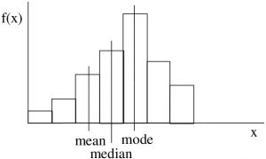
3.1.5 Mean, Median and Mode in Histograms: Skewness

If the shape of the histogram of a dataset is not too bizarre^[1] (e.g. unimodal) then we may determine the skewness of the dataset’s histogram (which would be a probability distribution of the data represented a population and not a sample) by comparing the mean or median to the mode. (Always compare something to the mode, no reliable information comes from comparing the median and mean.) If you have SPSS output with the skewness number calculated (we will see the formula for skewness later) then a left skewed distribution will have a negative skewness value, a symmetric distribution will have a skewness of 0 and, a right skewed distribution will have a positive skewness value.

Figure 3.1: A right skewed histogram (or distribution) generally has the mean and median to the right, or positive side of the mode. The tail of the histogram stretches to the right or positive side.

Symmetric distribution

Negatively skewed or left skewed histograms

Figure 3.3: A left skewed histogram (or distribution) generally has the mean and median to the left, or negative side of the mode. The tail of the histogram stretches to the left or negative side.

3.1.6 Mean, Median and Mode in Distributions: Geometric Aspects

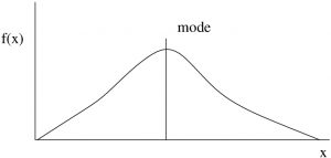
To understand the geometrical aspects of histograms we make the abstraction of letting the class widths shrink to zero so that the histogram curve becomes smooth. So let’s consider the mode, median and mean in turn.

Mode

The mode is the $x$ value where the frequency $f(x)$ is maximum, see Figure 3.4. More accurately the mode is a “local maximum” of the histogram^[2] (so if there are multiple modes, they don’t all have to have the same maximum value).

Median

The area under the curve is equal on either side of the median. In Figure 3.5 each area $A$ is the same. For relative frequencies (and so for probabilities) the total area under the curve is one. So the area on each side of the median is half. The median represents the 50/50 probability point; it is equally probable that $x$ is below the median as above it.

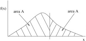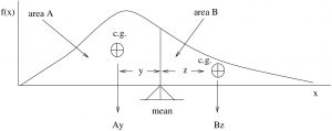
Mean

The mean is the balance point of the histogram/distribution as shown in Figure 3.6.

**A proof that the mean is the center of gravity of a histogram:

In physics, a moment is weight $\times$ moment arm :

$M = W x$

where $M$ is moment, $W$ is weight and $x$ is the moment arm (a distance).

Say we have two kids, kid1 and kid2 on a teeter-totter (Figure 3.7).

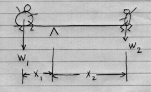
Kid1 with weight $W_{1}$ is heavy, kid2 with weight $W_{2}$ is light.

To balance the teeter-totter we must have

$W_{1} x_{1} = W_{2} x_{2}.$

The moment arm, $x_{1}$ , of the heavier kid must be smaller than the moment arm, $x_{2}$ , of the lighter kid if they are to balance.

So now let’s define the center of gravity. If you have a bunch of weights $W_{i}$ with corresponding moment arms $x_{i}$ then the center of gravity (c of g) is the moment arm $x_{g}$ (distance) that satisfies :

$\sum W_{i} x_{i} = W_{t} x_{g}$

where $W_{t} = \sum W_{i}$ is the total weight.

With histograms, instead of weight $W$ we have area $A$ . You can think of area as having a weight. (Think of cutting out a piece of the blackboard with a jigsaw after you draw a histogram on it.) So for a histogram (see Figure 3.8):

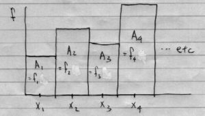
(We assume, for simplicity but “without loss of generality”, that $x_{i}$ are integers and also the classes. This is the case for discrete probability distributions as we’ll see.) So, for the c of g,

$\sum W_{i} x_{i} = W_{t} x_{g}$

translates to

$\sum A_{i} x_{i} = A_{t} x_{g}$

$\sum f_{i} x_{i} = (\sum f_{i} ) x_{g}$

$\sum f_{i} x_{i} = n x_{g}$

$x_{g} = \frac{\sum f_{i} x_{i}}{n}$

where we have used $A_{i} = f_{i}$ because the class widths are one, so

$x_{g} = \overline{x} = \frac{\sum f_{i} x_{i}}{n}.$

Because our “weight” is area, $\overline{x}$ is technically called the “1st moment of area”. (Variance, covered next, is the “2nd moment of area about the mean”.)

◻

For the purposes of deciding the skewness of a dataset in assignments and exams, you can assume that the histogram shape is not too bizarre. ↵
**In calculus terms, local maximums and minimums (and inflexion points) are where the derivative equals zero, $\frac{df}{dx}=0$ . ↵

License

Icon for the Creative Commons Attribution-NonCommercial-ShareAlike 4.0 International License

Introduction to Applied Statistics for Psychology Students Copyright © 2022 by Gordon E. Sarty is licensed under a Creative Commons Attribution-NonCommercial-ShareAlike 4.0 International License, except where otherwise noted.