
15. Chi Squared: Goodness of Fit and Contingency Tables
15.1 Goodness of Fit
For both the  goodness of fit and the contingency table tests, the test statistic is
![\[\chi^{2} = \sum_{i=1}^{C} \frac{(O_{i} - E_{i})^{2}}{E_{i}}\]](https://openpress.usask.ca/app/uploads/quicklatex/quicklatex.com-862a56cfda2a0a15a1c4fbae19fe699a_l3.png "Rendered by QuickLaTeX.com")
where
 = Observed frequency of category
  (the measurement)
 = Expected frequency of category (
 ).
).
 = number of categories.
For the goodness of fit test, the degrees of freedom for the critical statistic is  .
.
Limitation : In order for the test of frequencies to be valid (because of noise has a binomial distribution), all frequencies ( and
and  ) must be
  to be considered reliable.
Example 15.1 (Goodness of Fit example)
The advisor of an ecology club believes that the club consists of  freshmen,
  sophomores,
  juniors and
  seniors. The actual membership this year consisted of 14 freshmen, 19 sophomores, 51 juniors and 16 seniors. At
  test the advisor’s conjecture.
Solution :
0. Data reduction. Compute the observed and expected frequencies. In this example the total number of students is  so if we label the categories as :
category 1 = freshmen
category 2 = sophomores
category 3 = juniors
category 4 = seniors
then  ,
,  ,
,  ,
,  (converting percentages to frequencies)
and  ,
,  ,
,  ,
,  .
.
1. Hypotheses.

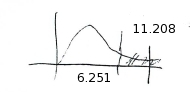
2. Critical statistic. Using the Chi-Square Distribution Table with (note that we only worry about the right tail as with  test statistics in ANOVA),
  we find
![\[ \chi^{2}_{\mbox{crit}} = 6.251 \]](https://openpress.usask.ca/app/uploads/quicklatex/quicklatex.com-e6dc9c5eed17a5b865a8ab4dba18d51a_l3.png "Rendered by QuickLaTeX.com")
3. Test statistic.

4. Decision.
Reject .
5. Interpretation. The advisor’s conjecture is wrong at . A plot of observed and expected frequencies (which we will plot as overlapping frequency polygons) shows how the observed frequencies are not a good fit to the expected frequencies :
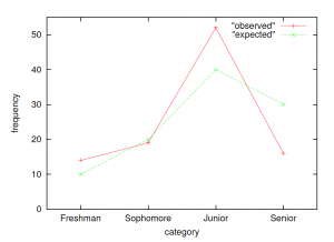
Here the fit of the data to the profile is not very good. If the fit between the observed frequencies (data) profile and the expected frequencies () profile is good, then will be small.
▢
15.1.1: Test of Normality using the Goodness of Fit Test
To test the hypotheses :
: The DV is normally distributed
 : The DV is not normally distributed
using the goodness of fit test[1] we first need to define the number of categories to use. The choice of how many categories to use is a bit of an art[2]. To work our way through the example below, we’ll take the category definition as a given. Then we’ll find that we’ll have to change that definition in order to have a valid test. This is how things will usually go in real life. The procedure for testing normality with a goodness of fit test is illustrated by example :
Example 15.2 : Suppose we have a dataset of 200 values of some measured DV. That is, suppose we have a sample of size  from a single population. Suppose further that
  DV
DV  . That is
  ,
,  and the range is
  . Let us (arbitrarily) divide the range into
  categories. Then (recall Chapter 2) the class width is
![\[ W = \frac{R+1}{G} = \frac{90}{6} = 15. \]](https://openpress.usask.ca/app/uploads/quicklatex/quicklatex.com-111429b4567a18a0ef4527595d43b91f_l3.png "Rendered by QuickLaTeX.com")
Suppose, finally, that the frequency table for the data is :
| Class | Class Boundaries | Frequency,  |
Midpoint,  |
 |
 |
| 1 | 89.5 — 104.5 | 24 | 97 | 2328 | 225,816 |
| 2 | 104.5 — 119.5 | 62 | 112 | 6944 | 777,728 |
| 3 | 119.5 — 134.5 | 72 | 127 | 9144 | 1,161,288 |
| 4 | 134.5 — 149.5 | 26 | 142 | 3692 | 524,264 |
| 5 | 149.5 — 164.5 | 12 | 157 | 1884 | 295,788 |
| 6 | 164.5 — 179.5 | 4 | 172 | 688 | 118,366 |
 = 200 = 200 |
 |
 |
At this point it will be useful for you to do a short exercise : Plot a histogram of this frequency table. If the data are normally distributed then the histogram will look approximately like a normal curve. The goodness of fit test that we will do quantifies this eyeball test.
Next, compute  and
and  using the sums from the table. Recall the group formulae :
![\[ \overline{x} = \frac{\sum f_{i} x_{m_{i}}}{n} = \frac{24680}{200} = 123.4 \]](https://openpress.usask.ca/app/uploads/quicklatex/quicklatex.com-1cf31178c1c214d8116d40a5c03abeb5_l3.png "Rendered by QuickLaTeX.com")
and

Now we are mostly ready to go through the goodness of fit hypotheses test :
0. Data reduction.
The frequency table for our data give the observed frequencies. Now we need to compute the expected frequencies by considering areas under the normal distribution that has the same mean,  , and standard deviation,
  , as our data. We’ll get those areas from the Standard Normal Distribution Table after
  -transforming our data. Once we have the area,
  , for each category , then we convert it to the expected frequency using
  . These calculations are completed in the following table where the -transforms of the category boundaries are computed using the usual
  . Notice that we used
  and
and  in place of the -transforms of
  and
and  just to catch the very tiny areas in the tails of the distribution. In the last column
  are copied from the data frequency table.
| Class | Class Boundaries | –transformed |
Standard Normal Distribution Table Areas | |
|
| 1 | 89.5 — 104.5 |  to -1.11 to -1.11 |
 |
26.7 | 24 |
| 2 | 104.5 — 119.5 | -1.11 to -0.23 |  |
55.1 | 62 |
| 3 | 119.5 — 134.5 | -0.23 to 0.65 |  |
66.64 | 72 |
| 4 | 134.5 — 149.5 | 0.65 to 1.53 |  |
38.96 | 26 |
| 5 | 149.5 — 164.5 | 1.53 to 2.41 |  |
11.0 | 12 |
| 6 | 164.5 — 179.5 | 2.41 to  |
 |
1.6 | 4 |
The areas on the distribution look like :
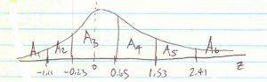
Recall that the goodness of fit test is valid only if all the frequencies are . The frequencies of class 6 are too low. As a quick fix, we’ll combine classes 5 and 6 into a new class 5. The class width of this new class will be twice that of the other classes but we can live with that. So, finally, the observed and expected frequencies that we’ll use for the hypothesis test are :
| Class |
|
|
| 1 | 26.7 | 24 |
| 2 | 55.1 | 62 |
| 3 | 66.64 | 72 |
| 4 | 38.96 | 26 |
| 5 | 12.6 | 16 |
1. Hypotheses.
: The population is normally distributed.
: The population os not normally distributed.
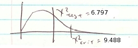
2. Critical statistic.
From the Chi-Square Distribution Table with  and
and  find
find
![\[ \chi^{2}_{\mbox{crit}} = 9.488 \]](https://openpress.usask.ca/app/uploads/quicklatex/quicklatex.com-8f2e7f09d947ad3592b12ff0768f5057_l3.png "Rendered by QuickLaTeX.com")
3. Test statistic.

4. Decision.
Do not reject .
5. Interpretation. The population appears to be normally distributed.
▢
- This is a test of the assumptions that might underlie a test of interest. This test, like most hypotheses tests applied to test assumptions, will find the desired assumption to be true when you fail to reject . There are other tests for normality that we don't cover in this course. One of the more popular tests for normality is the Komolgorov-Smirnov test for comparing distributions. ↵
- The choice of how many categories to choose for making a histogram is in general a wide open question. ↵
