
14.5 Flooding
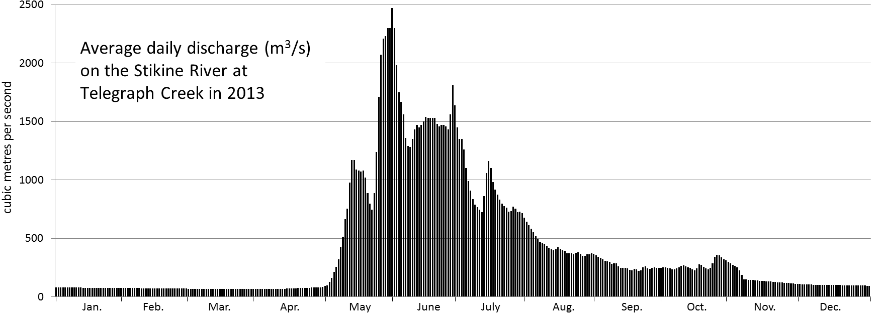
The discharge levels of streams are highly variable depending on the time of year and on variations in the weather from one year to the next. In Canada, most streams show discharge variability similar to that of the Stikine River in northwestern BC, illustrated in Figure 14.26. The Stikine River has its lowest discharge levels in the depths of winter when freezing conditions persist throughout most of its drainage basin. Discharge starts to rise slowly in May, and then rises dramatically through the late spring and early summer as the winter snow melts. For the year shown, the minimum discharge of the Stikine River was 56 m3/s in March, and the maximum was 37 times higher at 2,470 m3/s in May.
![Figure 13.24 Variations in discharge of the Stikine River during 2013. [SE from data at Water Survey of Canada, Environment Canada, http://www.ec.gc.ca/rhc-wsc/]](http://opentextbc.ca/geology/wp-content/uploads/sites/110/2015/08/Stikine-River.png)
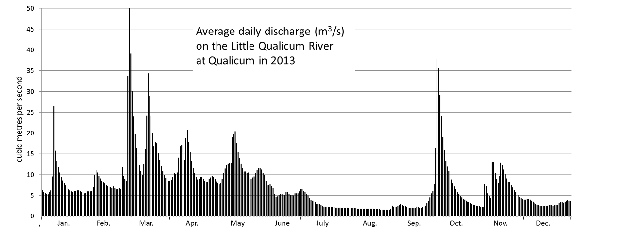
Streams in coastal areas of southern British Columbia show a very different pattern from those in most of the rest of the country. In this region, the drainage basins receive a lot of rain (rather than snow) during the winter and also do not remain entirely frozen throughout the winter. The Qualicum River on Vancouver Island typically has its highest discharge levels in January or February and its lowest levels in late summer (Figure 14.27). In 2013, the minimum discharge of the Qualicum River was 1.6 m3/s in August, and the maximum was 34 times higher at 53 m3/s in March.
![Figure 13.25 Variations in discharge of the Qualicum River during 2013. [SE from data at Water Survey of Canada, Environment Canada, http://www.ec.gc.ca/rhc-wsc/]](http://opentextbc.ca/geology/wp-content/uploads/sites/110/2015/08/Qualicum-River.png)
When a stream’s discharge increases, both the water level (stage) and the velocity increase as well. Rapidly flowing streams become muddy, and large volumes of sediment are transported both in suspension and along the stream bed. In extreme situations, the water level reaches the top of the stream’s banks (the bank-full stage, see Figure 14.19), and if it rises further, it will overflow the banks and floods the surrounding terrain. In the case of mature or old-age streams, this could include a vast area of relatively flat ground known as a flood plain, which is the area that is typically covered with water during a major flood. Since fine river sediments are deposited on flood plains, they are ideally suited for agriculture, and thus are typically occupied by farms and residences, and in many cases, by towns or cities. Such infrastructure is highly vulnerable to damage from flooding, and the people that live and work there are at risk.
Most streams in Canada have the greatest risk of flooding in the late spring and early summer when stream discharges rise in response to melting snow. In some cases, this is exacerbated by spring storms. In years when melting is especially fast and/or spring storms are particularly intense, flooding can be very severe.
One of the worst floods in Canadian history took place in the Fraser Valley of BC in late May and early June of 1948. The early spring of that year had been cold, and a large snow pack in the interior was slow to melt. In mid-May, temperatures rose quickly and melting was accelerated by rainfall. Fraser River discharge levels rose rapidly over several days during late May, and the dykes built to protect the valley were breached in a dozen places. Approximately one-third of the flood plain was inundated, and many homes and other buildings were destroyed, but there were no deaths.
The Fraser River flood of 1948, which was the worst flood in the Fraser Valley in the past century, was followed by very high river levels in 1950 and 1972, and by relatively high levels several times since then, the most recent being 2007 (Table 13.1). In the years following 1948, millions of dollars were spent repairing and raising the existing dykes and building new ones. Since then damage from flooding in the Fraser Valley has been relatively limited.
| Rank | Year | Month | Date | Stage (m) | Discharge (m3/s) |
| 1 | 1948 | May | 31 | 11.0 | 15,200 |
| 2 | 1972 | Jun | 16 | 10.1 | 12,900 |
| 3 | 1950 | Jun | 20 | 9.9 | 12,500 |
| 4 | 1964 | Jun | 21 | 9.6 | 11,600 |
| 5 | 1997 | Jun | 5 | 9.5 | 11,300 |
| 6 | 1955 | Jun | 29 | 9.4 | 11,300 |
| 7 | 1999 | Jun | 22 | 9.4 | 11,000 |
| 8 | 2007 | Jun | 10 | 9.3 | 10,850 |
| 9 | 1974 | Jun | 22 | 9.3 | 10,800 |
| 10 | 2002 | Jun | 21 | 9.2 | 10,600 |
Table 14.1 Ranking of the maximum stage and discharge values for the Fraser River at Hope between 1948 and 2008. Typical discharge levels are ~1,000 m3/s. Source: Data from Mannerstrom (2008) Comprehensive Review of Fraser River at Hope Flood Hydrology and Flows Scoping Study, Report prepared for the B.C. Ministry of the Environment. view source
Serious flooding occurred in July 1996 in the Saguenay-Lac St. Jean region of Quebec. In this case, the floods were caused by two weeks of heavy rainfall followed by one day of exceptional rainfall. On July 19, 1996 there was 270 mm of rain, equivalent to the region’s normal rainfall for the entire month of July. Ten deaths were attributed to the Saguenay floods, and the economic toll was estimated at $1.5 billion.
Just a year after the Saguenay floods, the Red River in Minnesota, North Dakota, and Manitoba reached its highest level since 1826. As is typical for the Red River, the 1997 flooding was due to rapid snowmelt. Due to the south to north flow of the river, the flooding starts in Minnesota and North Dakota, where melting begins earlier, then extends northwards. The residents of Manitoba had plenty of warning that the 1997 flood was coming because there was severe flooding at several locations on the U.S. side of the border.
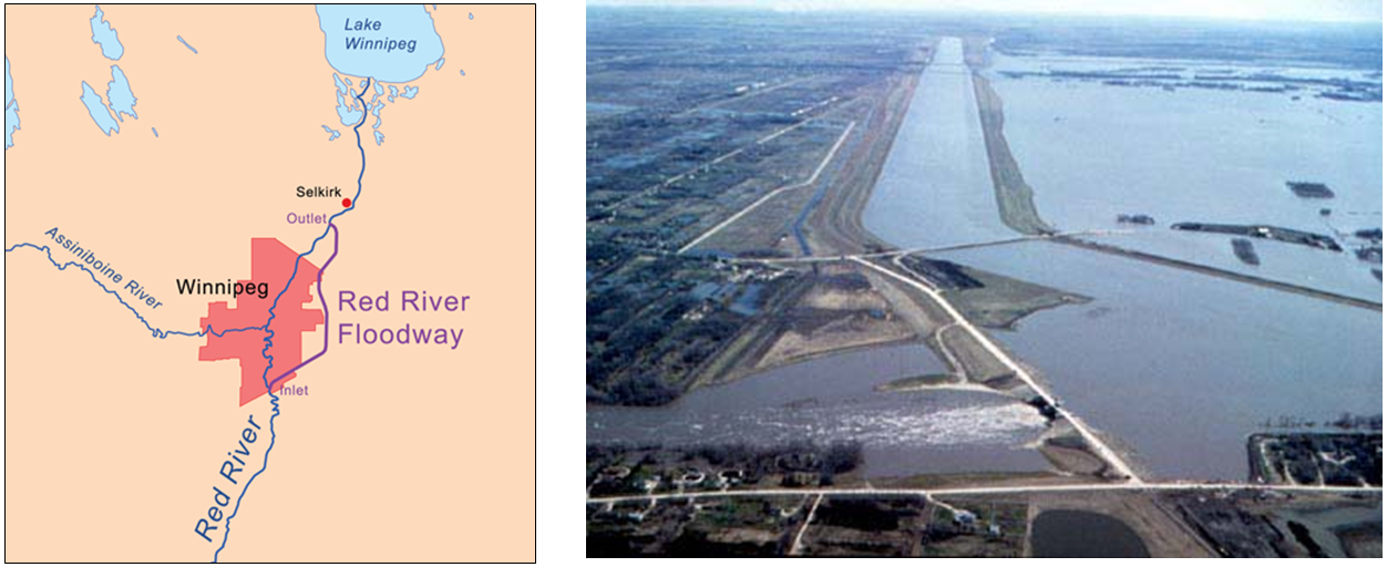
After the 1950 Red River flood, the Manitoba government built a channel around the city of Winnipeg to reduce the potential of flooding in the city (Figure 14.28). Known as the Red River Floodway, the channel was completed in 1964 at a cost of $63 million. Since then it has been used many times to alleviate flooding in Winnipeg, and is estimated to have saved many billions of dollars in flood damage. The massive 1997 flood (Figure 14.28, right side) was almost too much for the floodway; in fact the amount of water diverted was greater than the designed capacity. The floodway has recently been expanded so that it can be used to divert even more of the Red River’s flow away from Winnipeg.
![Figure 13.26 Map of the Red river Floodway around Winnipeg, Manitoba (left), and aerial view of the southern (inlet) end of the floodway (right). [Map from http://en.wikipedia.org/wiki/1997_Red_River_Flood#/media/File:Rednorthfloodwaymap.png and photo from Natural Resources Canada 2012, courtesy of the Geological Survey of Canada (Photo 2000-118 by G.R. Brooks).]](http://opentextbc.ca/geology/wp-content/uploads/sites/110/2015/08/Red-river-Floodway.png)
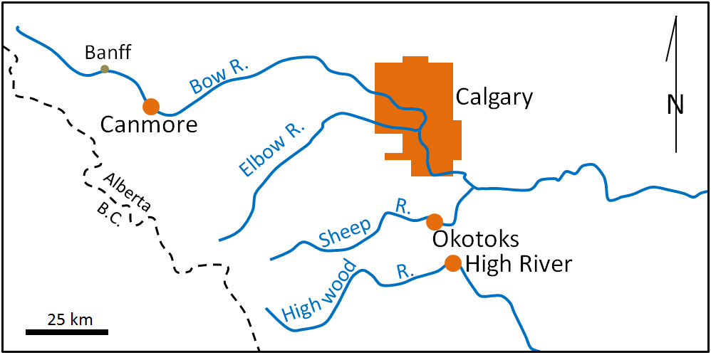
Canada’s most costly flood ever was the June 2013 flood in southern Alberta. The flooding was initiated by snowmelt and worsened by heavy rains in the Rockies due to an anomalous flow of moist air from the Pacific and the Caribbean. At Canmore, AB rainfall amounts exceeded 200 mm in 36 hours, and at High River, AB 325 mm of rain fell in 48 hours.
![Figure 13.27 Map of the communities most affected by the 2013 Alberta floods (in orange) [SE]](http://opentextbc.ca/geology/wp-content/uploads/sites/110/2015/08/Alberta-floods.png)
In late June and early July, the discharges of several rivers in the area, including the Bow River in Banff, Canmore, and Exshaw, the Bow and Elbow Rivers in Calgary, the Sheep River in Okotoks, and the Highwood River in High River, reached levels that were 5 to 10 times higher than normal for that time of year (see Exercise 14.5). Large areas of Calgary, Okotoks, and High River were flooded, and five people died (see Figures 14.29 and 14.30). The cost of the 2013 flood is estimated to be approximately $5 billion.
![Figure 13.28 Flooding in Calgary (June 21, left) and Okotoks (June 20, right) during the 2013 southern Alberta flood [http://upload.wikimedia.org/wikipedia/commons/6/6a/Riverfront_Ave_Calgary_Flood_2013.jpg http://upload.wikimedia.org/wikipedia/en/9/9b/Okotoks_-_June_20%2C_2013_-_Flood_waters_in_local_campground_playground-03.JPG]](http://opentextbc.ca/geology/wp-content/uploads/sites/110/2015/08/Flooding-in-Calgary.png)
One of the things that the 2013 flood of the Bow River teaches us is that we cannot predict when a flood will occur nor how big it will be, so in order to minimize damage and casualties we need to be prepared. Some ways of preparing include:
- Mapping flood plains and not building within them
- Building dykes or dams where necessary
- Monitoring the winter snowpack, the weather, and stream discharges
- Creating emergency plans
- Educating the public on how to prepare for and respond to the threat of flooding
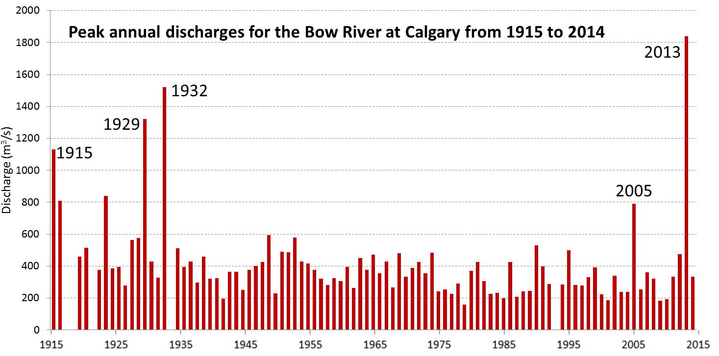
Exercise 14.5 Flood Probability on the Bow River
The graph below shows the highest discharge per year between 1915 and 2014 of the Bow River in Calgary. Using this data set, we can calculate the recurrence interval (Ri) for any particular flood magnitude using the equation: Ri = (n+1)/r (where n is the number of floods in the record being considered, and r is the rank of the particular flood). There are a few years missing in this record, so the actual number of floods is 95.
The largest flood recorded along the Bow River over that period of time was the one in 2013, reaching a peak flow rate of 1,840 m3/s on June 21. Ri for this flood is (95+1)/1 = 96 years. The probability of such a flood in any future year is 1/Ri x 100%, which is 1%. The fifth largest flood was just a few years earlier in 2005, at 791 m3/s. Ri for this flood is (95+1)/5 = 19.2 years. The recurrence probability of a flood of this magnitude is thus 5%.
- Calculate the recurrence interval for the second largest flood (1932, 1,520 m3/s).
- What is the probability that a flood of 1,520 m3/s will happen next year?
- Examine the 100-year trend for floods along the Bow River. If you ignore the major floods (the labelled ones), what is the general trend of peak discharges over this time?
