7.3 Thévenin’s Theorem

Samuel J. Ling; Jeff Sanny; William Moebs; Daryl Janzen

7.3 Thévenin’s Theorem

LEARNING OBJECTIVES

By the end of the section, you will be able to:

Find the Thévenin equivalent circuit for any linear circuit
Calculate the maximum power that can be transferred to a load at any point in a circuit, and the value of the load resistance required to draw maximum power

Thévenin’s theorem states that any linear circuit containing several voltage sources and resistors can be simplified to a Thévenin-equivalent circuit with a single voltage source and resistance connected in series with a load. Specifically, the three components connected in series are (see Figure 7.3.1(b)):

Load resistor, $R_L$ ;
Thévenin voltage $V_{\mathrm{th}}$ , found by removing $R_L$ from the original circuit and calculating the potential difference from one load connection point to the other (e.g. from $a$ to $b$ in Figure 7.3.1(a), either across $R_1,$ $V_1,$ and $R_3$ or across $R_2$ and $R_3$ );
Thévenin resistance $R_{\mathrm{th}}$ , found by removing $R_L$ from the original circuit and calculating the total equivalent resistance between the two load connection points (e.g. between $a$ and $b$ in Figure 7.3.1(a), thus as the equivalent resistance of the parallel combination of $R_1$ and $R_2$ , connected in series with $R_3$ ).

(Figure 7.3.1) $\begin{gather*}.\end{gather*}$

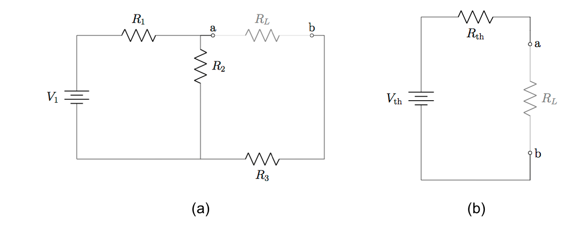**Figure 7.3.1** (a) An example of a DC resistive circuit with load resistor $R_L$ identified, and (b) its Thévenin equivalent. In fact, (b) shows the general form of all Thévenin-equivalent circuits.

Thévenin’s theorem is particularly useful when the load resistance in a circuit is subject to change. When the load’s resistance changes, so does the current it draws and the power transferred to it by the rest of the circuit. In fact, currents everywhere in a circuit will be subject to change whenever a single resistance changes, and the entire circuit would need to be re-analysed to find the new current through and power transferred to a load. Repeating circuit analysis to find the new current through a load every time its resistance changes would be very time-consuming. In contrast, according to Thévenin’s theorem once $V_{\mathrm{th}}$ and $R_{\mathrm{th}}$ are determined for the rest of the circuit, the current through the load is always simply calculated as

(7.3.1) $\begin{equation*}I_L=\frac{V_{\mathrm{th}}}{R_{\mathrm{th}}+R_L},\end{equation*}$

from which the voltage drop across, and power transferred to the load are, respectively,

(7.3.2) $\begin{equation*}V_L=R_LI_L=\frac{R_LV_{\mathrm{th}}}{R_{\mathrm{th}}+R_L},\end{equation*}$

(7.3.3) $\begin{equation*}P_L=I_L^2R_L=\frac{V_L^2}{R_L}=\frac{R_LV_{\mathrm{th}}^2}{(R_{\mathrm{th}}+R_L)^2.}\end{equation*}$

Equations 7.3.1–7.3.3 are easily applied, and the problem of repeated circuit analysis each time a load’s resistance changes is mainly reduced to the one-time problem of finding the Thévenin voltage $V_{\mathrm{th}}$ and resistance $R_{\mathrm{th}}$ with respect to $R_L$ . Example 7.3.1 shows the procedure for doing this for the circuit in Figure 7.3.1(a).

EXAMPLE 7.3.1

Applying Thévenin’s Theorem

Find $V_{\mathrm{th}}$ and $R_{\mathrm{th}}$ for the circuit in Figure 7.3.1(a).

Strategy

Find $V_{\mathrm{th}}$ : note that with the circuit open between $a$ and $b$ there is no current through, and therefore no voltage drop across $R_3$ . Therefore, the potential difference between $a$ and $b$ must occur in the loop containing $V_1,$ $R_1,$ and $R_2.$ We are free to choose either parallel branch of that loop, as the potential difference across $R_2$ must equal the potential difference across $V_1$ and $R_1$ by the loop rule. Therefore, we will first determine the current in this loop and apply Ohm’s law to find $V_{\mathrm{th}}=V_{R_2}$ .
Find $R_{\mathrm{th}}$ : Proceeding from $a$ to $b$ we encounter a junction where the circuit branches in two directions, towards $R_1$ and $R_2$ . $V_1$ is an ideal voltage source with no resistance, and can therefore be ignored when calculating equivalent resistance. We then encounter another junction where the two branches reconnect, so $R_1$ and $R_2$ are connected in parallel. Proceeding on, we encounter $R_3$ in series with the parallel connection of $R_1$ and $R_2$ , and eventually reach $b$ . We will add these resistances using the rules for adding series and parallel resistors.

Solution

The current through the loop with $V_1$ , $R_1$ and $R_2$ all connected in series is

$I=\frac{V_1}{R_1+R_2}.$

By Ohm’s law, the voltage across $R_2$ is therefore

$V_{R_2}=R_2I=\frac{R_2V_1}{R_1+R_2}.$

By our above reasoning, we therefore have

$V_{\mathrm{th}}=V_{R_2}=\frac{R_2V_1}{R_1+R_2}.$

To find $R_{\mathrm{th}},$ first write

$R_{12}=\left(\frac{1}{R_1}+\frac{1}{R_2}\right)^{-1}=\frac{R_1R_2}{R_1+R_2}.$

Then, by our above reasoning,

$R_{\mathrm{th}}=R_{12}+R_3=\frac{R_1R_2}{R_1+R_2}+R_3.$

Significance

The potential difference from $a$ to $b$ was calculated as a drop in potential across $R_2$ as current flows from the positive to the negative terminal of the voltage source $V_1.$ Along the parallel branch (that is, parallel from the perspective of the load connection points $a$ and $b$ ), potential rises at $V_1$ , then drops across $R_1$ , travelling in the clockwise direction. By the loop rule, there must be an overall potential rise in the clockwise direction along this branch that equals negative the potential drop in the clockwise direction across $R_2$ . Thus, between $a$ and $b$ along the left branch, travelling in the counter-clockwise direction there is also a drop in potential, equal to

$-(V_1-R_1I)=-V_1+\frac{R_1V_1}{R_1+R_2}=\frac{R_2V_1}{R_1+R_2}=R_{\mathrm{th}},$

as required.

It is important to note that perspective matters when treating components as being connected in series or parallel. Here, when determining the current through $R_2$ in the open circuit, we noted that current flows through a single circuit loop with $V_1,$ $R_1,$ and $R_2$ all connected in series, and determined the current through $R_2$ as the potential drop across the series combination of resistors, divided by the equivalent resistance. However, when calculating $R_{\mathrm{th}}$ we found that from the perspective of the connection points $R_1$ and $R_2$ are connected along parallel branches of the circuit.

The procedure used here to calculate $V_{\mathrm{th}}$ and $R_{\mathrm{th}}$ is the same as that which we apply to more complex circuits. When doing so, it is important to correctly account for voltage rises and drops across between the two load connection points, although to this end we do have freedom of choice in which branch to follow and can always choose the simplest path.

CHECK YOUR UNDERSTANDING 7.3

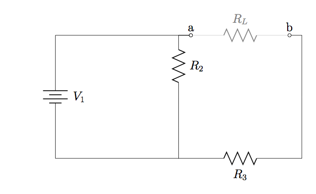
The circuit is the same as the one from Example 7.3.1, but with $R_1$ replaced by a short. Determine $V_{\mathrm{th}}$ and $R_{\mathrm{th}}$ in this case.

Maximum Power Transfer Theorem

Thévenin’s theorem finds a useful application in the maximum power transfer theorem, which states that maximum power will be transferred to a load when its resistance is equal to the Thévenin resistance of the network supplying the power. This interesting and highly useful fact is easily proven by taking the derivative of Equation 7.3.3 with respect to $R_L$ , setting the result equal to $0$ , and solving for the value of $R_L$ that maximises the function.

$\frac{dP_L}{dR_L}=\frac{V_{\mathrm{th}}^2}{(R_{\mathrm{th}}+R_L)^2}-\frac{2R_LV_{\mathrm{th}}^2}{(R_{\mathrm{th}}+R_L)^3}=0$

$\Rightarrow 1-\frac{2R_L}{R_{\mathrm{th}}+R_L}=0$

$\Rightarrow R_L=R_{\mathrm{th}}.$

EXAMPLE 7.3.2

Applying Maximum Power Transfer Theorem

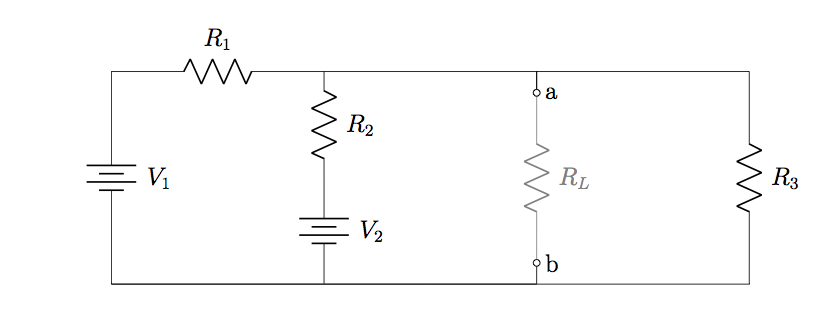
What is the maximum amount of power that can be dissipated in $R_L$ ?

**Figure 7.3.2** A DC resistive network.

Strategy

The maximum amount of power that can be dissipated in $R_L$ is, by the maximum power transfer theorem, the power dissipated when $R_L=R_{\mathrm{th}},$ for the Thévenin equivalent circuit calculated with respect to $R_L.$ To find this, we first determine $V_{\mathrm{th}}$ and $R_{\mathrm{th}},$ as follows.

With $R_L$ replaced by an open circuit, there are two loops: one, passing through $V_1,$ $R_1,$ $R_2,$ and $V_2;$ the other, passing through $V_2,$ $R_2,$ and $R_3$ . We will calculate the current through $R_3$ using Mesh Analysis techniques developed earlier, then determine $V_{\mathrm{th}}=V_{R_3}$ using Ohm’s law. Note that we do not actually need to calculate any other currents, since $V_{\mathrm{th}},$ the potential difference between $a$ and $b,$ must equal $V_{R_3}$ regardless which branch is taken.

To find $R_{\mathrm{th}}$ , note that with respect to connection points $a$ and $b$ , $R_1,$ $R_2,$ and $R_3$ are all connected in parallel.

Finally, when $R_L=R_{\mathrm{th}},$ the current in the load is $I_L=V_{\mathrm{th}}/2R_{\mathrm{th}}$ (see Equation 7.3.1), and the power dissipated in $R_L$ is $P_{L,\mathrm{max}}=I_L^2R_L=V_{\mathrm{th}}^2/4R_{\mathrm{th}}$ (cf. Equation 7.3.3).

Solution

Using the strategies developed in Mesh Analysis, we can write the matrix equations for this network as

$\left(\begin{array}{c}-V_1+V_2\\-V_2\end{array}\right)=\left(\begin{array}{cc}-(R_1+R_2)&R_2\\R_2&-(R_2+R_3)\end{array}\right)\left(\begin{array}{c}I_1\\I_2\end{array}\right),$

where $I_1$ and $I_2$ are the clockwise mesh currents in the left and right loops, respectively.

To find $I_2$ (the actual current in $R_3$ ), we apply Cramer’s rule:

$\begin{eqnarray*}I_2&=&\frac{\left|\begin{array}{cc}-(R_1+R_2)&-V_1+V_2\\R_2&-V_2\end{array}\right|}{\left|\begin{array}{cc}-(R_1+R_2)&R_2\\R_2&-(R_2+R_3)\end{array}\right|}=\frac{V_2R_1+V_2R_2+V_1R_2-V_2R_2}{R_1R_2+R_2^2+R_1R_3+R_2R_3-R_2^2}\\&=&\frac{V_2R_1+V_1R_2}{R_1R_2+R_1R_3+R_2R_3}.\end{eqnarray*}$

The Thévenin-equivalent voltage is therefore

$V_{\mathrm{th}}=R_3I_2=\frac{R_3(V_2R_1+V_1R_2)}{R_1R_2+R_1R_3+R_2R_3}.$

The Thévenin-equivalent resistance is

$R_{\mathrm{th}}=\left(\frac{1}{R_1}+\frac{1}{R_2}+\frac{1}{R_3}\right)^{-1}=\frac{R_1R_2+R_1R_3+R_2R_3}{R_1R_2R_3}.$

Finally, the maximum power dissipated in $R_L,$ when $R_L=R_{\mathrm{th}}$ , is

$P_{L,\mathrm{max}}=\frac{V_{\mathrm{th}}^2}{4R_{\mathrm{th}}}=\frac{R_1R_2R_3^3(V_2R_1+V_1R_2)^2}{(R_1R_2+R_1R_3+R_2R_3)^3}.$

Significance

It is important to be clear that $P_{L,\mathrm{max}}$ is the power dissipated in $R_L$ only when $R_L=R_{\mathrm{th}}.$ The general expression for power dissipated in $R_L$ is given by Equation 7.3.3.

License

Icon for the Creative Commons Attribution 4.0 International License