
7.1 Mesh Analysis
LEARNING OBJECTIVES
- Write simultaneous linear equations in matrix form
- Apply techniques of linear algebra to solve for current vector
- Solve linear circuits by advanced mesh analysis methods
Kirchhoff’s rules of circuit analysis—at any junction, the sum of incoming currents equals the sum of outgoing currents; and, the potential difference around a closed loop is zero—are the necessary and sufficient conditions for determining the current through each component of any linear circuit—that is, any circuit composed only of elements that respond linearly to changes in current or voltage (such as Resistors, Capacitors and Inductors). Thus, the problem-solving strategy you learned in Kirchhoff’s Rules is sufficient to analyse any such circuit. However, that approach is inefficient and its steps are prone to human error—problems we’d like to mitigate in particular when applying the basic principles of circuit analysis to more complex circuits.
The mesh analysis techniques you learn in this section will not necessarily advance your knowledge of the physics of electrical circuits. Rather, the objective of this section is to provide a simpler and more straightforward approach to the analysis of planar circuits (also known as “meshes”). By the end of this section, you will see that it is possible to determine the current in all branches of a circuit in two easy steps: read off the components of a vector  and a matrix
  simply by observation; solve for the vector of mesh currents
  . But before this useful result can be realised, we must first explore a few nuanced points to explain why the technique works.
We begin by modifying the problem-solving strategy from Kirchhoff’s Rules, adding a few particular requirements and removing some unneeded steps.
Problem-Solving Strategy: Mesh Analysis
- Draw mesh current loops, ensuring:
- each loop is unique; and
- all circuit elements—voltage sources, resistors, capacitors, inductors, etc. and short circuits—are covered by at least one loop.
- Apply loop rule as described in Kirchhoff’s Rules (particularly with reference to Figure 6.3.5) and solve simultaneous equations.
- Add or subtract mesh currents in branches that are covered by multiple loops, depending on the direction of each loop and the sign of each current calculated in step 2.
Referring back to the problem-solving strategy described in Kirchhoff’s Rules, you should see that we have removed three steps and replaced them with step 3 here. Rather than defining arbitrary currents at each junction, then using the loop rule to eliminate some of the current variables, we now skip straight to defining current loops, apply the loop rule, and solve directly for each mesh current. Then, as these may turn out to be positive or negative depending on the direction of the loops chosen arbitrarily in step 1, we add or subtract values as appropriate in branches covered by multiple mesh currents to find the actual current through each.
The tradeoff results in a small complication in step 2, which effectively absorbs the junction rule into the way we must apply the loop rule. However, when dealt with in a consistent manner (as we will do here) this is a minor complication.
Let us compare approaches by revisiting the problem from Example 6.3.1.
EXAMPLE 7.1.1
Calculating Current by the Mesh Analysis Approach
Find the currents flowing in the circuit in Figure 7.1.1.
(Figure 7.1.1) 
Strategy
Referring to the mesh analysis problem-solving strategy above:
- Note that the mesh currents
 and
and  :
:
- are unique (i.e.
 ), and
 - pass through every circuit element.
- are unique (i.e.
- Applying the loop rule means adding all the voltage rises and drops around each loop and setting the sum equal to zero. For each voltage source, and for each resistor encountered by only one mesh current, this is a straightforward application of the rules given by the map in Figure 6.3.5. But when more than one mesh current passes through a resistor, as with
 in this example, in each loop equation we must account for the fact that each mesh current contributes to the potential difference. Thus, e.g. in the case of
  the potential difference at is written as
  (there is a voltage drop across due to pointing in the direction of travel around loop , and a voltage rise due to pointing opposite the direction of travel).
 - After solving simultaneous equations, we may find that or is negative, which would indicate that our initial choice of direction was incorrect. In fact, we know from Example 6.3.1 that points in the right direction and points in the wrong direction. Thus, the actual current—as opposed to our arbitrarily-defined mesh currents—is to the right in both the top and bottom branches, and to the left in the centre branch of the circuit. The actual current in the centre branch will therefore have magnitude

Solution
Applying the loop rule yields the following two equations for the unknown mesh currents, and :

And rearranging terms, we find
(7.1.1) 
Solving (e.g. multiplying the second equation by  , adding the result to the first and solving for ) yields the expected result for the two mesh currents:
![\[I_1=0.20~\mathrm{A},~~~I_2=-0.30~\mathrm{A}.\]](https://openpress.usask.ca/app/uploads/quicklatex/quicklatex.com-238e64bd4d83732044b780d0b6047845_l3.png "Rendered by QuickLaTeX.com")
Thus, the current in the bottom branch of the circuit must be  to the right, the current in the top branch must be
  to the right, and the current in the centre branch must be
  to the left.
Significance
We have arrived at the same result as in Example 6.3.1. This is not surprising, as the approach taken here is in fact mathematically equivalent to our previous approach.
However, we have simplified things by skipping the steps of labelling nodes, defining currents into and out of each junction, and applying the junction rule. In doing so, we’ve reduced the number of simultaneous equations that need to be solved, by precisely the number resulting from application of the junction rule (in this case, we went from three equations to two).
Skipping steps as we have done resulted in the following complication: when applying the loop rule, for the resistor that is adjacent to both loops, we picked up a term for the potential difference with respect to the loop, and a term  for the potential difference with respect to the loop. The reason for this is simple: we have absorbed application of the junction rule into our application of the loop rule—i.e. both of Kirchhoff’s rules still generally apply in our analysis, we’ve just adjusted our approach. Thus, instead of defining a third current
  , applying the junction rule to obtain
  , then substituting into our loop rule expressions, we skip right to applying the loop rule for each mesh current and solve the system of fewer equations with fewer unknown variables.
Matrix Operations for Linear Circuit Analysis: Cramer’s Rule
Any system of linear equations can be written in matrix form, and by doing so one is able to apply techniques of linear algebra to efficiently compute solutions. For example, the system of equations found in Equation 7.1.1 can be rewritten as
(7.1.2) 
In general, the system of equations for an  -loop circuit will have the form
  , where and
  are -dimensional column vectors and is an
  -matrix. When and are known, the elements of can be computed explicitly through a formula discovered by Gabriel Cramer (1704-1752), known as Cramer’s rule:
(7.1.3) 
where  is the
  -th element of and
  is the matrix formed by replacing the -th column of with .
EXAMPLE 7.1.2
Applying Cramer’s Rule
Calculate the solution to the problem in Example 7.1.1 using Cramer’s rule.
Strategy
Apply Cramer’s rule (Equation 7.1.3) to the matrices in Equation 7.1.2 to determine the values of and .
Solution
![\[I_1=\frac{\mathrm{det}(\mathbf{R}_1)}{\mathrm{det}(\mathbf{R})}=\frac{\left|\begin{array}{cc}-1.10~\mathrm{V}&1~\Omega\\2.90~\mathrm{V}&-9~\Omega\end{array}\right|}{\left|\begin{array}{cc}-4~\Omega&1~\Omega\\1~\Omega&-9~\Omega\end{array}\right|}=\frac{9.90~\mathrm{V}\cdot\Omega-2.90~\mathrm{V}\cdot\Omega}{36~\Omega^2-1~\Omega^2}=0.20~\mathrm{A},\]](https://openpress.usask.ca/app/uploads/quicklatex/quicklatex.com-50e98dd70af42b36c5f27c7799aa1910_l3.png "Rendered by QuickLaTeX.com")
![\[I_2=\frac{\mathrm{det}(\mathbf{R}_2)}{\mathrm{det}(\mathbf{R})}=\frac{\left|\begin{array}{cc}-4~\Omega&-1.10~\mathrm{V}\\1~\Omega&2.90~\mathrm{V}\end{array}\right|}{\left|\begin{array}{cc}-4~\Omega&1~\Omega\\1~\Omega&-9~\Omega\end{array}\right|}=\frac{-11.6~\mathrm{V}\cdot\Omega+1.10~\mathrm{V}\cdot\Omega}{35~\Omega^2-1~\Omega^2}=-0.30~\mathrm{A}.\]](https://openpress.usask.ca/app/uploads/quicklatex/quicklatex.com-2dfe66b3c55bc367af86ef80c563f0e0_l3.png "Rendered by QuickLaTeX.com")
Significance
Cramer’s rule indeed yields our previous result. The main advantage of this approach is the straightforward application of a rule that always provides an explicit result. The only requirement is that the rules for defining mesh current loops stated in the above problem-solving strategy are followed. In contrast, if identical mesh current loops were defined, the rows of would not be linearly independent and will be singular; and if the chosen loops did not cover all circuit elements, important information would be missing and the result would be incorrect.
Cramer’s rule is a very handy rule, particularly for students in test-situations, or for engineers working in the field who do not have access to computers. However, Cramer’s rule is computationally very inefficient for systems of more than three equations, so is generally not very useful for solving circuits with more than three loops. In that case, computer programs like MATLAB that can quickly invert matrices are very useful, as you will see below.
A Procedure for Reading and Directly from the Circuit
When working with many systems of equations, writing out equations with many terms whose signs depend on repeated application of a few rules, and rearranging terms to write those equations in a particular form, human error can be difficult to avoid. A useful strategy for mitigating such errors is to find a consistent simplifying procedure. Indeed, as we will now see, a very useful pattern becomes apparent simply by always drawing mesh current loops that all point in the same direction.
To begin, let us revisit what happened when writing the -terms in the loop equations of Example 7.1.1. For both loops, the potential difference at had the form  , where
  was the mesh current in the loop of interest and
  was the adjacent mesh current. Indeed, in general when all the mesh current loops of a circuit are defined as pointing in the same direction—i.e. either clockwise or counterclockwise—the potential differences across all resistors
  located between adjacent mesh current loops are
  , where is the mesh current in the loop of interest and is the adjacent mesh current.
This is already a useful observation for mesh analysis, as it leads to the following set of rules for writing loop equations. Note that these rules can be used only when mesh current loops are defined as all pointing in the same direction. In this case, for any mesh current loop  the potential difference across every voltage source and resistor will be:
 when flows through voltage source from negative to positive,
 when flows through voltage source from positive to negative,
 when only flows through resistor
  , and
, and- when and an adjacent mesh current loop both flow through .
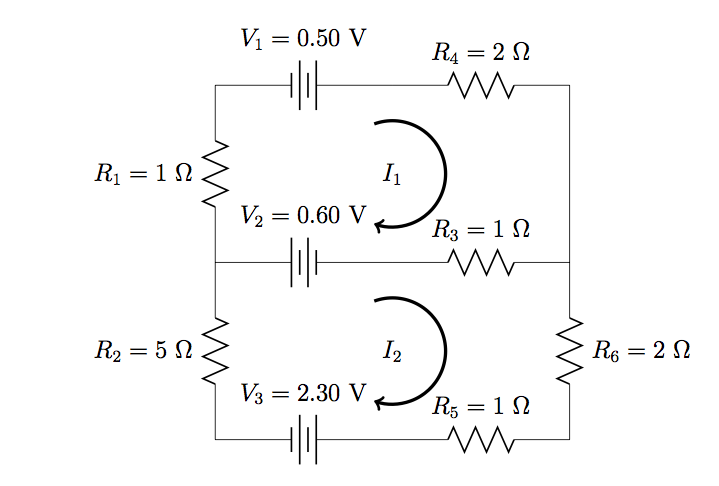
While this set of rules may be useful, it is just one step towards a more useful result we will now observe upon applying these rules to write down the matrix equations for a reasonably large, five loop-circuit in Example 7.1.3. Namely, through this example we will observe a general set of rules to follow for “reading” the and matrices directly from the circuit diagram.
EXAMPLE 7.1.3
Matrix Equation of a Five Loop-Circuit
Write down the and -matrices for the circuit in Figure 7.1.2.
(Figure 7.1.2) 
Strategy
Write the five loop equations by applying the four rules above to each resistor and voltage source in the circuit. Subtract voltage terms from each side, and factor each current variable from up to five terms (one for each mesh current). Write the linear system of equations in matrix form.
Solution
The five mesh current loop equations are:

Rearranging terms, we find
![\[\begin{array}{rccccc}V_1=&-(R_1+R_3+R_4)I_1&+R_1I_2&+R_3I_3&+R_4I_4&+0,\\V_2=&R_1I_1&-(R_1+R_2)I_2&+0&+0&+0,\\-V_2=&R_3I_1&+0&-(R_3+R_5)I_3&+0&+R_5I_5,\\-V_3=&R_4I_1&+0&+0&-R_4I_4&+0,\\V_3=&0&+0&+R_5I_3&+0&-R_5I_5.\end{array}\]](https://openpress.usask.ca/app/uploads/quicklatex/quicklatex.com-a3ceecbb15787a416e6719f4d274fe5f_l3.png "Rendered by QuickLaTeX.com")
Therefore,
![\[\mathbf{V}=\left(\begin{array}{c}V_1\\V_2\\-V_2\\-V_3\\V_3\end{array}\right)\]](https://openpress.usask.ca/app/uploads/quicklatex/quicklatex.com-48133dc72561b3d8d8b84ff0ed5150ad_l3.png "Rendered by QuickLaTeX.com")
![\[\mathbf{R}=\left(\begin{array}{ccccc}-(R_1+R_3+R_4)&R_1&R_3&R_4&0\\R_1&-(R_1+R_2)&0&0&0\\R_3&0&-(R_3+R_5)&0&R_5\\R_4&0&0&-R_4&0\\0&0&R_5&0&-R_5\end{array}\right)\]](https://openpress.usask.ca/app/uploads/quicklatex/quicklatex.com-8ec42b1dccf88a02e8f9b630f12c1c59_l3.png "Rendered by QuickLaTeX.com")
Significance
When rearranging terms in the second step, a term was added explicitly for each mesh current, including  for each term not actually part of the sum, in anticipation of the next step.
Note the following patterns in the and matrices:
 is negative the sum of voltage rises and drops due to voltage sources around each mesh current loop .
 is negative the sum of the resistances of the resistors around mesh current loop .
 is the sum of resistances of the resistors through which any mesh current loop adjacent to also passes.
We need to be careful not to draw conclusions too generally, as these patterns do not necessarily follow from the general mesh analysis procedure. Rather, this particular pattern is the result of two additional steps taken here: (i) all current loops were defined as pointing in the same direction (i.e. clockwise), and (ii) when rearranging loop equations the variables due to voltage sources were moved to the left-hand side of each loop equation, thus writing each loop equation in the form “negative of voltage supplied around each loop equals sum of voltage drops across resistors.”
Neither step (i) nor (ii) is required for mesh analysis. For example, mesh current is allowed to be defined as pointing in the other direction, in which case all terms in column would be multiplied by  . Similarly, the equation for loop could instead be rearranged in the form “voltage supplied around each loop equals negative the sum of voltage drops across resistors.” In this case, both and row would be multiplied by .
Because of the differences that could exist in the signs of terms in and , it should be clear that without a consistent approach to mesh analysis it is very easy to make sign errors. In contrast, by choosing one approach and sticking with it, we see at once a clear pattern, i.e. the above list of three points, for reading the terms of and directly from the circuit.
The significance of our final observation in Example 7.1.3 is a great simplification to the computational procedure of mesh analysis. However, these simplifying steps are not strictly necessary, as circuit analysis can proceed very well by following the steps developed in Kirchhoff’s Rules which are more closely associated with the physics of electrical circuits. For instance, we must be careful not to draw any physical significance from the description of two opposing mesh currents flowing through a circuit branch; at the macroscopic level, there is only one real current in each branch, which is the sum of all mesh currents there.
Therefore, rather than gaining any further physical insight, here we have developed a straightforward procedure to minimise the number of steps and the potential for human error in the analysis of planar circuits. This result is so useful that we restate it here explicitly.
PROCEDURE FOR READING AND DIRECTLY FROM THE CIRCUIT
- Draw one mesh current loop inside each loop of the circuit.
- Work your way around each loop , reading off terms and as follows:
- is the sum
 for each voltage source
 that passes from negative to positive, and
  for each voltage source
 that passes through from positive to negative,
 - is the sum
 for each resistor
 that passes, and
 is the sum
  for each resistor
 passed by a loop adjacent to .
CHECK YOUR UNDERSTANDING 7.1
Apply the above procedure to read off the terms of and directly from the following circuits. Note that you can check your results (and demonstrate the great simplification afforded by the procedure just stated) by following the steps taken in Example 7.1.3.
With our mesh analysis methods now in hand, it is time for a final example demonstrating the most common application: read the circuit matrices directly from the circuit, and use a computer to solve for the mesh currents.
EXAMPLE 7.1.4
Complete Circuit Analysis in Two Steps with MATLAB
Calculate the currents through each of the resistors and voltage sources in the circuit of Figure 7.1.3, and use the results to find the power dissipated by all resistors and power supplied by all voltage sources.
(Figure 7.1.3) 
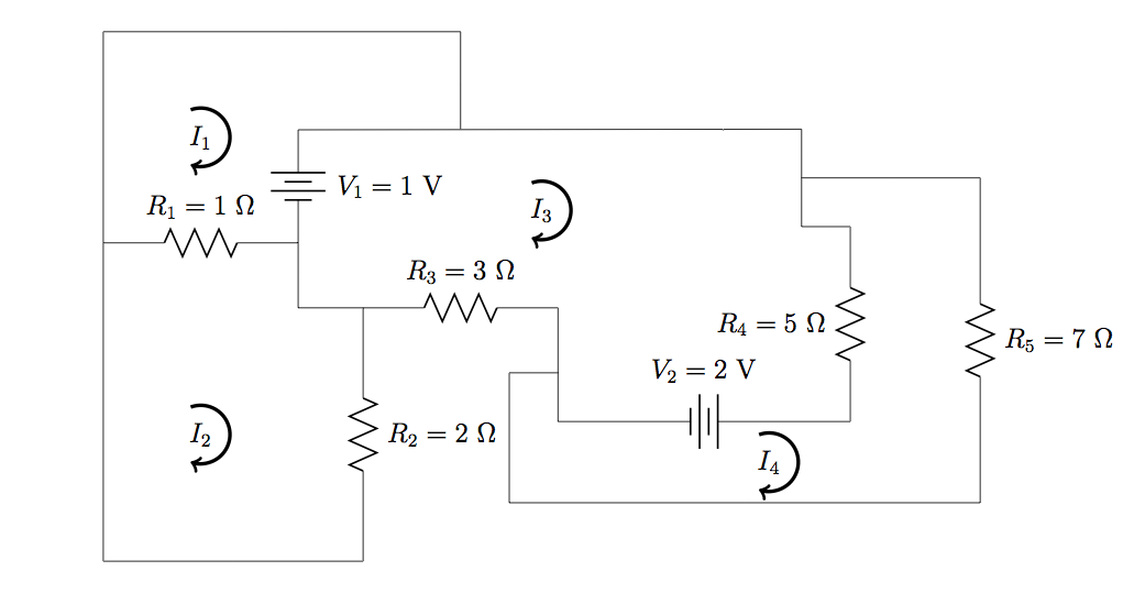
Strategy
Apply the procedure for reading and directly from the circuit. For simplicity, disregard units inside the matrices, noting that the mesh currents in will have units of amps. Use MATLAB to calculate . Add or subtract results as appropriate to find the actual currents through each component of the circuit. Calculate power dissipated by resistors as  and power supplied by voltage sources as
Solution
![\[\mathbf{V}=\left(\begin{array}{c}V_1\\0\\-V_1+V_2\\-V_2\end{array}\right)=\left(\begin{array}{c}1\\0\\1\\-2\end{array}\right)\]](https://openpress.usask.ca/app/uploads/quicklatex/quicklatex.com-200135a92631acb2130d8714d5fccf6b_l3.png "Rendered by QuickLaTeX.com")

Figure 7.1.3 shows the MATLAB code and output solution for 
(Figure 7.1.4) 
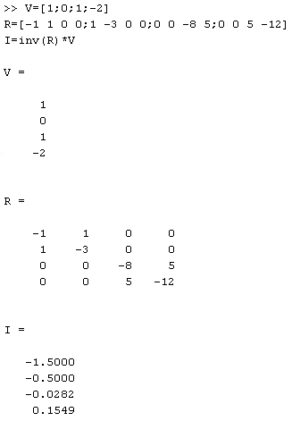
The components of can be used to compute the current through each component of the circuit. Thus, we find:
 to the right,
 upward,
 to the right,
 upward,
 downward,
 upward.
The power supplied by the voltage sources is
![\[P_{\mathrm{supplied}}=\sum_iI_{V_i}V_i=1.4718~\mathrm{W}+0.3662~\mathrm{W}=1.8380~\mathrm{W},\]](https://openpress.usask.ca/app/uploads/quicklatex/quicklatex.com-bb66ea0c9c46a83b7c0ccc1a96d0f0a3_l3.png "Rendered by QuickLaTeX.com")
and the power dissipated over the resistors is

Significance
By following the steps of mesh analysis developed in this section, analysis of planar circuits is straightforward. For two- and three-loop circuits, Cramer’s rule provides a quick means to calculate by hand; for circuits with four loops or more, it is best to use a computer to quickly calculate 
Candela Citations
- Authored by: Daryl Janzen. Provided by: Department of Physics & Engineering Physics, University of Saskatchewan. License: CC BY: Attribution
