
Chapter 10. Water
Overview of Water
Adapted by Joyce M. McBeth (2018) University of Saskatchewan from Deline B, Harris R, & Tefend K. (2015) “Laboratory Manual for Introductory Geology”. First Edition. Chapter 5 “Water” by Randa Harris, CC BY-SA 4.0. View Source. Last updated: 14 July 2020.
10.2 STREAMFLOW AND PARTS OF A STREAM
The running water in a stream will erode (wear away) and move material within its channel, including dissolved substances (materials taken into solution during chemical weathering). The solid sediments may range in size from tiny clay and silt particles too small for the naked eye to view up to sand and gravel sized sediments. Even boulders have been carried by large flows. The smaller particles kept in suspension by the water’s flow are called suspended load. The dissolved substances in the water are called dissolved load. Larger particles typically travel as bed load. The bed load rolls, slides, and salts (hops) along the stream bed (Figure 10.1). While the dissolved, suspended, and bed loads may travel long distances (e.g., from the headwaters of the Bow River in the Rocky Mountains to the mouth of the Saskatchewan River where it discharges into Lake Winnipeg), they will eventually settle out, or deposit. These stream deposited sediments, called alluvium, can be deposited at any time, but most often occur during flood events. To more effectively transport sediment, a stream needs energy. This energy is mostly a function of the amount of water and its velocity (speed), as more (and larger) sediment can be carried by a fast-moving stream. As a stream loses its energy and slows down, material will be deposited.
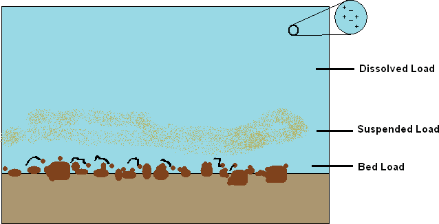
Source: PSUEnviroDan (2008) public domain view source
Under normal conditions, water will remain in a stream channel. When the amount of water in a stream exceeds its banks, the water that spills over the edges of the channel decreases in velocity rapidly. As the water velocity drops, the water will also drop the larger sandy material it is carrying right along the channel margins, resulting in ridges of sandy alluvium called natural levees (Figure 10.2). As numerous flooding events occur, these ridges build up under repeated deposition. These levees are part of a larger landform known as a floodplain. A floodplain is the relatively flat land adjacent to the stream that is subject to flooding during times of high discharge.
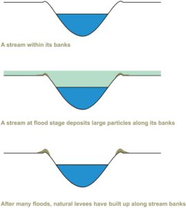
Source: Julie Sandeen (2009) CC BY-SA 3.0 view source
10.2.1 Stream Drainage Basins and Patterns
The drainage basin (also known as watershed, catchment area, or river basin) of a stream includes all the land that is drained by the stream and all of its tributaries (the smaller streams that feed into the main stream). Small drainage basins are part of larger drainage basins (e.g., the drainage basin for a small mountain stream will be part of the drainage basin for the river it flows into). You are in a drainage basin right now. Do you know which one? Search for images of “drainage basin” or “watershed” and your province on the internet to find information on your local watersheds. For example, if you live in Saskatchewan you can refer to the Saskatchewan Water Security Agency’s map of watersheds in Saskatchewan.
At the continental scale, ocean watersheds drain the runoff from large regions of the continents into oceans. There are five ocean watersheds in Canada: the Arctic Ocean watershed, the Pacific Ocean watershed, the Hudson Bay watershed, the Atlantic Ocean watershed, and a small part of southern Alberta and Saskatchewan drains into the Gulf of Mexico watershed.
The higher areas that separate drainage basins are called drainage divides. Drainage divides can be very high topographically (e.g.; the Great Divide in the Rockies which separates drainage to the Pacific Ocean in the west from drainage to the Arctic Ocean, Hudson Bay, the Atlantic Ocean, and the Gulf of Mexico) or lower (e.g., the Arctic Divide that runs through Alberta, Saskatchewan, the NWT, and Nunavut, dividing drainage to the Arctic Ocean from drainage to Hudson Bay).
Water erodes softer rocks more easily than it erodes hard, resistant rock. This can result in characteristic patterns of drainage. Some of the more common drainage patterns include:
- Dendritic – this drainage pattern indicates uniformly resistant bedrock that often includes horizontal rocks. Since all the rock is uniform, the water does not erode any area preferentially; thus, the channels form a branching pattern similar to the branches of a tree.
- Trellis – this drainage pattern indicates alternating resistant and non-resistant bedrock that has been deformed (folded) into parallel ridges and valleys. The water erodes the softer rock, and the channels that develop from erosion appear much like a rose climbing on a trellis in a garden.
- Radial – this drainage pattern forms as streams flow away from a central high point, such as a volcano, and the pattern resembles the spokes in a wheel.
- Rectangular – this drainage pattern forms in areas in which rock has been fractured or faulted which created weakened rock. Streams erode the less resistant rock and create a network of channels that make right-angle bends as they intersect these breaking points. This pattern will often look like rectangles or squares.
- Deranged – this drainage pattern does not follow any of the patterns above, it is a random pattern of irregular stream channels. Deranged drainage patterns are found where drainage developed recently and has not yet had time to form one of the other drainage patterns.
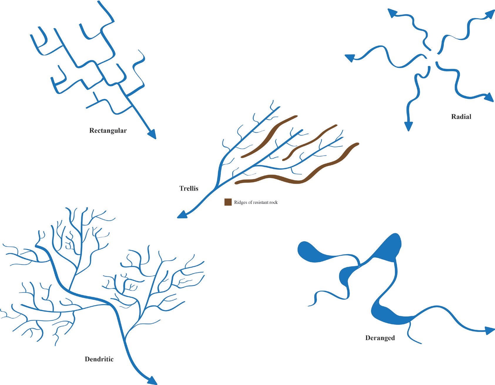
Source: Corey Parson (2015) CC BY-SA 3.0 view source
10.3 STREAM GRADIENT AND THE CYCLE OF STREAM EROSION
Stream gradient refers to the slope of the stream’s channel. It is the vertical drop of the stream over a horizontal distance (the rise and run, respectively). You have dealt with gradient before in Topographic Maps. The gradient can be calculated using the following equation:
Gradient = (change in elevation) / distance
Let’s calculate the gradient from A to B in Figure 10.4 below. The elevation of the stream at A is 980 m, and the elevation of the stream at B is 920 m. Using the scale bar on the figure, we calculate the distance from A to B is 2 km. Gradient = (980 m – 920 m) / 2 km, or 30 m/km.

Source: Joyce McBeth (2018) CC BY-SA 4.0, after Randa Harris (2015) CC BY-SA 3.0 view source
Stream gradients tend to be higher in a stream’s headwaters (where it originates), and lower at the stream’s mouth (where it discharges into another body of water such as the ocean). Discharge measures stream flow at a given time and location; it is a measure of the volume of water passing a particular point in a given period of time. It is found by multiplying the area (width multiplied by depth) of the stream channel by the velocity of the water, and is often in units of cubic meters per second. Discharge increases downstream in most rivers, as tributaries join the main channel and add water.
Sediment load (the amount of sediment carried by the stream) also changes from the stream’s headwaters to its mouth. At the headwaters, tributaries quickly carry their load downstream, combining with loads from other tributaries. The main river then eventually deposits that sediment load when it reaches base level (the point where the stream is at the same elevation as a lake or ocean that it discharges into).
Sometimes in this process of carrying material downstream, the sediment load is large enough that the water cannot support it, so deposition occurs. If a stream becomes overloaded with sediment, braided streams may develop, with a network of intersecting channels that resembles braided hair. Sand and gravel bars are typical in these braided streams. Braided streams are common in regions with abundant sediments and variable discharge, for example in streams that discharge from glaciers.
Straight streams are less common; these stream channels remain nearly straight due to a linear zone of weakness in the underlying rock (e.g., a fault). They are common near the headwaters of streams in mountainous regions, where the stream flows in a generally straight line through steep-sided canyons. Straight channels can also be man-made, to help with flood control.
Meandering streams have broadly looping curves that resemble an “S”-shape. These are known as meanders (Figure 10.5). The water traveling in a meandering stream moves fastest on the outside bends of the stream. This greater velocity and turbulence from the faster flow lead to more erosion on these outside bends, forming a featured called a cut bank (a bank with a steep slope). Erosion on this bank is offset by deposition on the opposite bank of the stream, where slower moving water allows sediment to settle out. These deposits are called point bars.
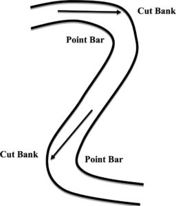
Source: Randa Harris (2015) CC BY-SA 3.0 view source
As meanders become more complicated, or sinuous, they may cut off another meander in the stream. When this happens, the cut off meander becomes a crescent-shaped oxbow lake (Figure 10.6).
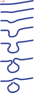
Source: User Maksim on Wikimedia Commons (2005) CC BY-SA 2.5 view source
Even though streams are not living, they do go through characteristic changes over time as they change the landscape. Ultimately, streams will reach base level. This is the low elevation at which the stream can no longer erode its channel – often a lake or other stream. The ultimate base level is the ocean. Over a stream’s evolution, it will experience a cycle of stream erosion, which consists of these stages (Figure 10.7):
- Youthful (early) stage – these streams are downcutting their channels (vertically eroding), picking up sediment from the bottom of their channels and decreasing their elevation. The land surface will be above sea level, and these streams form deep V-shaped channels.
- Mature (middle) stage – these streams experience both vertical (downcutting) and lateral (meandering) erosion. The land surface is sloped, and streams begin to form floodplains (the flat land around streams that are subject to flooding).
- Old age (late) stage – these streams erode laterally rather than vertically (i.e., they move by meandering across the landscape) and have very complicated meanders and oxbow lakes. The land surface is near base level.
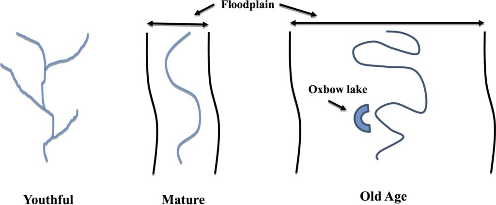
Source: Randa Harris (2015) CC BY-SA 3.0 view source
An interruption may occur in this cycle. If the base level drops (e.g., due to a drop in sea level) the stream will begin to downcut again. This can also occur if the area around it was uplifted (think building mountains). If the stream was in the old age stage when this change in base level or uplift occurred, it will begin to form a deep V-shaped channel within that complicated meandering pattern that it has. This creates a neat geologic feature called an entrenched meander (Figure 10.8).
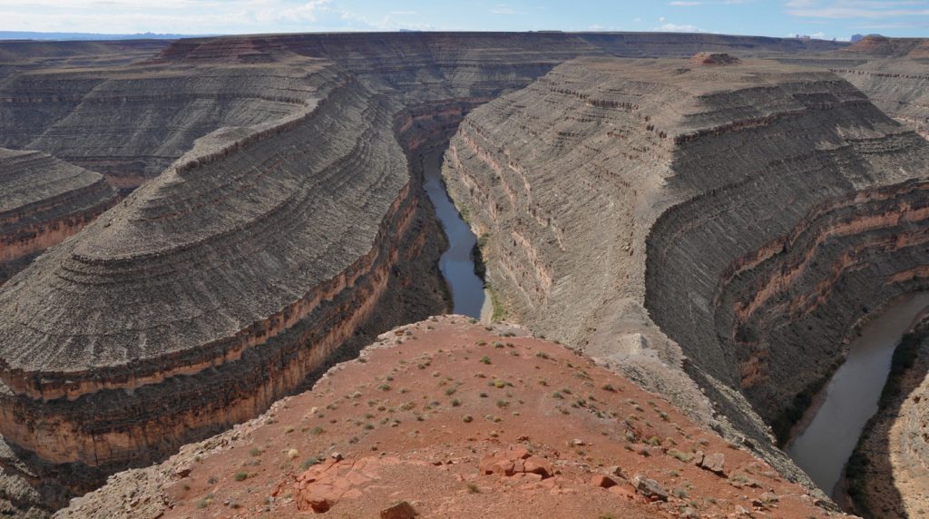
Source: User “Finetooth” (2010) CC BY-SA 3.0 view source
10.4 FLOODING
Flooding is a common and serious problem globally. Flood stage is reached when the water level in a stream overflows its banks. Floodplains are evidence for past flooding of a stream. Floodplains are also popular sites for development: they have nice water views and are flat and composed of sediments that are easy to landscape. Perhaps these areas are best left for playgrounds and golf courses if you consider the potential damage that a flood might do to buildings and property.
When we describe flood risk, we often describe the risk frequency in terms such as “1 in 100 year flood”. How often do you think a 1 in 100 year flood will occur? Does it mean that a flood of similar magnitude will occur every 100 years? Not necessarily! It means that – on average – we can expect a flood of this size or greater to occur within a 100 year period. One cannot predict that it will occur in a particular year, only that each year has a 1 in 100 chance of having a flood of that magnitude. It also does not mean that only one flood of that size can occur within 100 years. The “1 in 100 year flood” is based on previous historical and geological records, so if the climate of a region is experiencing change over time (e.g., if there is more rainfall in a mountainous region over a period of several years where in previous decades it was arid) the flooding frequency may be higher than that predicted using the historical data.
In order to better understand stream behavior, Environment Canada has installed thousands of stream gauges across the country to record water level and stream discharge. Data from these stations can be used to make flood frequency curves, which are useful in making flood control decisions.
A major flood event on the Bow and Elbow rivers that run through Calgary, Alberta occurred in June 2013 (Figure 10.9). The flood resulted in an estimated $5 billion in property damage, one of the most costly natural disasters in Canadian history. In the days before the flood, the region west of Calgary received rainfall far above seasonal averages. Over 100,000 people were evacuated due to the flooding and five people died. While this was a catastrophic event, it is important to note that there are numerous dams upstream of Calgary that normally regulate the flow of water and prevent major flooding events. Historically, major floods were more common in Calgary than they are today. Other major floods in Canada include the Red River flood in Manitoba in 1997, and the Fraser River flood in B.C. in 1894.
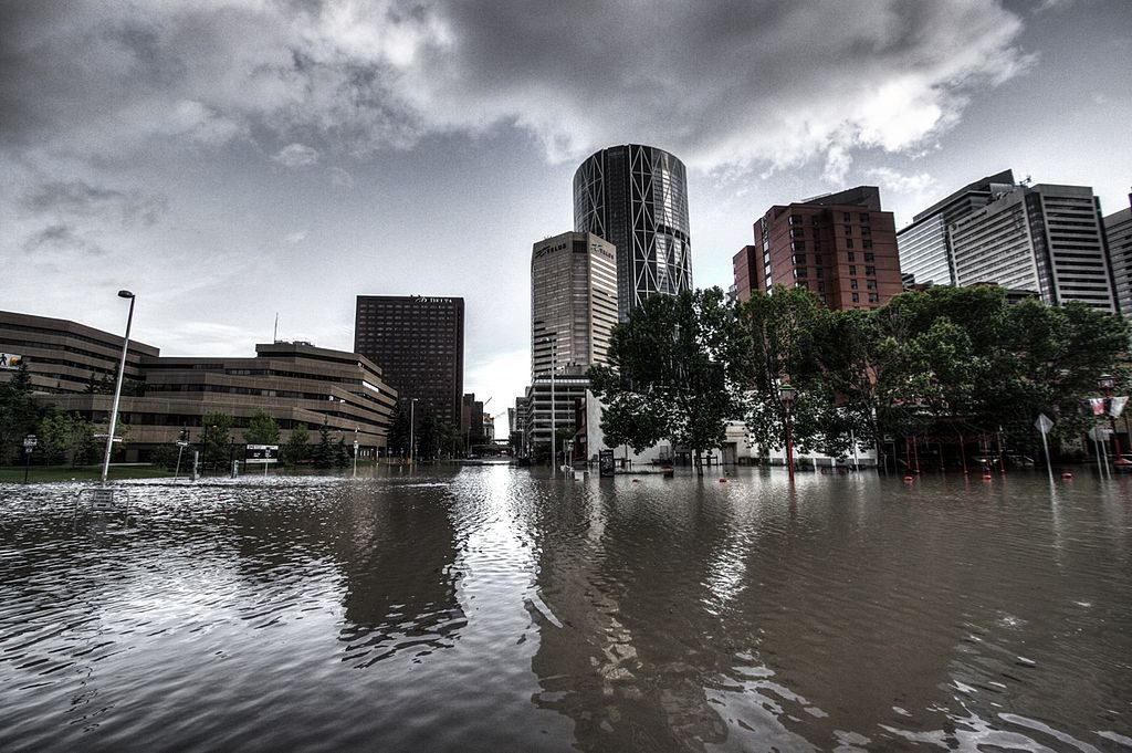
Source: Flickr user Ryan Quan (2013) CC BY-SA-NC view source
10.5 GROUNDWATER
It is best not to envision groundwater as underground lakes and streams (which only occasionally exist in caves). Instead, think of groundwater as water slowly seeping from one miniscule pore in the rock to another, or along fractures in the rock. Have you ever been to the beach and dug a hole, only to have it fill with water from the base? If so, you were looking at the water table, the boundary between the unsaturated and saturated zones in the beach sediments (Figure 10.10). Rocks and soil just beneath the land’s surface (and above the water table) are part of the unsaturated zone, and the pore spaces in these rocks are filled with air. Once the water table is reached, then rocks and soil pore spaces are filled with water; this is the saturated zone.
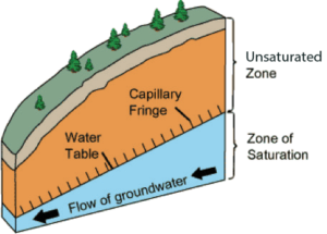
Source: USGS (2011) Public Domain view source
The water table is said to mimic topography, in that it generally lies near the surface of the ground. It is often within a few metres below the surface, though this can vary greatly with location depending on factors such as the rock type and the amount of regional precipitation. The water table rises with hills and sinks with valleys, often intersecting with the surface to discharge into streams. It receives additional inputs as rainfall infiltrates into the ground, called recharge. Its position is dynamic – during droughts (periods of low rainfall) the water table will lower and when it is rainier it will rise.
Two important properties of aquifers that influence groundwater availability and movement are porosity and permeability. Porosity refers to the open or void space within the aquifer rock or sediments. Porosity is the percentage of the total rock volume composed of open spaces. Porosity will vary with rock type. Many rocks with tight interlocking crystals (such as igneous and metamorphic rocks) generally have low porosity since they lack open spaces between the mineral crystals. Sedimentary rocks composed of well sorted sediment tend to have high porosity because of the abundant spaces between the grains that make them up. If these spaces are filled with cement sedimentary rocks may have low porosity.
To visualize porosity, envision a room filled from floor to ceiling with basketballs (this is analogous to a rock composed completely of sand grains). Now add water to the room. The room will be able to hold a good deal of water, since the basketballs don’t pack tightly due to their shape. That would be an example of high porosity.
Permeability refers to the ability of a geologic material to transport fluids. It depends upon the porosity within the rock, but also on the size of the open space and how interconnected those open spaces are. Even though a material is porous, if the open spaces aren’t connected, water won’t flow through it. Rocks that are permeable make good aquifers, geologic units that are able to yield significant water. Sedimentary rocks such as sandstone and limestone are generally good aquifers. Rocks that are impermeable make confining layers and prevent the flow of water. Examples of confining layers would be sedimentary rocks like shale (made from tiny clay and silt grains) or unfractured igneous or metamorphic rock. In an unconfined aquifer, where there is no confining geological layer above the aquifer, the top of the aquifer is the water table.
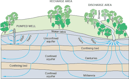
Groundwater generally flows from areas of higher elevation to lower elevation in the shallow subsurface (Figure 10.11). About 30% of the population of Canada uses groundwater as their source of drinking water. Groundwater can be contaminated which is a threat to this resource. Common sources of contamination include sewage, landfills, industry, and agriculture. The movement of groundwater helps spread the pollutants, making containment a challenge.
10.6 KARST TOPOGRAPHY
The sedimentary rock limestone is composed of the mineral calcite, which is water soluble, meaning it will dissolve in water that is weakly acidic. In humid areas where limestone is found, water dissolves the rock, forming large cavities and depressions which vary in size and shape. As more dissolution occurs, the caves become unstable and collapse, creating sinkholes. These broad, crater-like depressions are typical of karst topography (Figure 10.12), named after the Karst region in Slovenia. Karst topography is characterized by sinkholes, sink lakes (sinkholes filled with water), caves, and disappearing streams (surface streams that disappear into a sinkhole).

Source: Randa Harris (2015) CC BY-SA 3.0 view source
Living in karst topography poses challenges for building infrastructure; sinkholes can appear rather rapidly and cause great damage to any structures above them. In Canada, there are examples of karst across the country aside from on the Canadian Shield. For example, there is karst topography in Wood Buffalo National Park and near Norman Wells, NWT (Figure 10.13) and in southern Ontario.
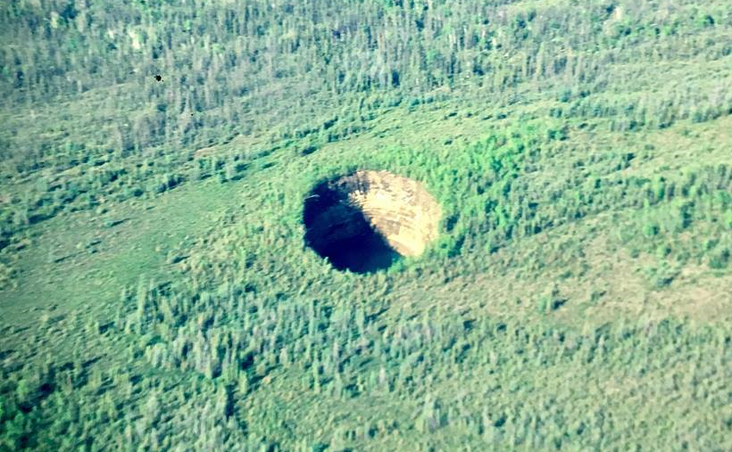
Source: Dennis McBeth (1994) CC BY-SA 4.0.
