
Chapter 7. Topographic Maps
Exercises on Topographic Maps
Adapted by Joyce M. McBeth, Sean W. Lacey, & Tim C. Prokopiuk (2018) University of Saskatchewan from Deline B, Harris R, & Tefend K. (2015) “Laboratory Manual for Introductory Geology”. First Edition. Chapter 3 “Topographic Maps” by Karen Tefend and Bradley Deline, CC BY-SA 4.0. View Source.
The purpose of this lab is to familiarize students with how to read and use topographic maps. This is a critical skill to prepare students to learn about more complex geologic maps. Note: the maps used in this lab are in colour and the colours have significance in terms of the symbols and patterns used on the maps – it is best to print this lab in colour and from a pdf version.
Name: _______________
Student number: ____________
Date and lab section time: _____________
TAs’ names: _______________ _______________
Please hand in this lab to your TAs at the end of the lab period.
Links to maps used in this lab
- British Columbia Topographic Map 092G095. https://pub.data.gov.bc.ca/datasets/177864/pdf/092G/092G095.pdf
- Saskatoon topographic map: https://openpress.usask.ca/app/uploads/sites/52/2018/08/SKtopomap_v2.pdf
7-E2 LAB EXERCISE – TOPOGRAPHIC MAPS
This is a graded activity, please submit it to your TA at the end of the lab. Note: This lab is in colour. Therefore, if you print it out in black and white please refer back to the electronic copy to avoid confusion. For all of the following figures, assume north is at the top of the map, and south at the bottom.
Questions 1 to 9: basic topographic map skills
Overview section 7.3 provides background information on contour lines to prepare you for these exercises.
1. (5 pts) The following topographic map (Map 7-E3) is from a coastal area and features an interesting geological hazard in addition to the ocean. Using a contour interval of 40 m, label the elevation of every contour line on the map below. Note: elevation is metres above sea level; thus, sea level = ______ m
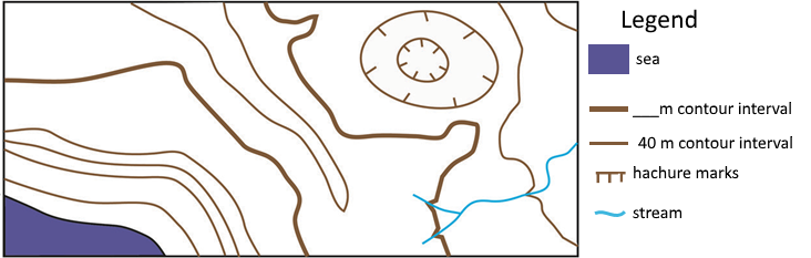
Source: Joyce M. McBeth (2018) CC BY-SA 4.0, after Brad Deline (2017) CC BY-SA 3.0 view source
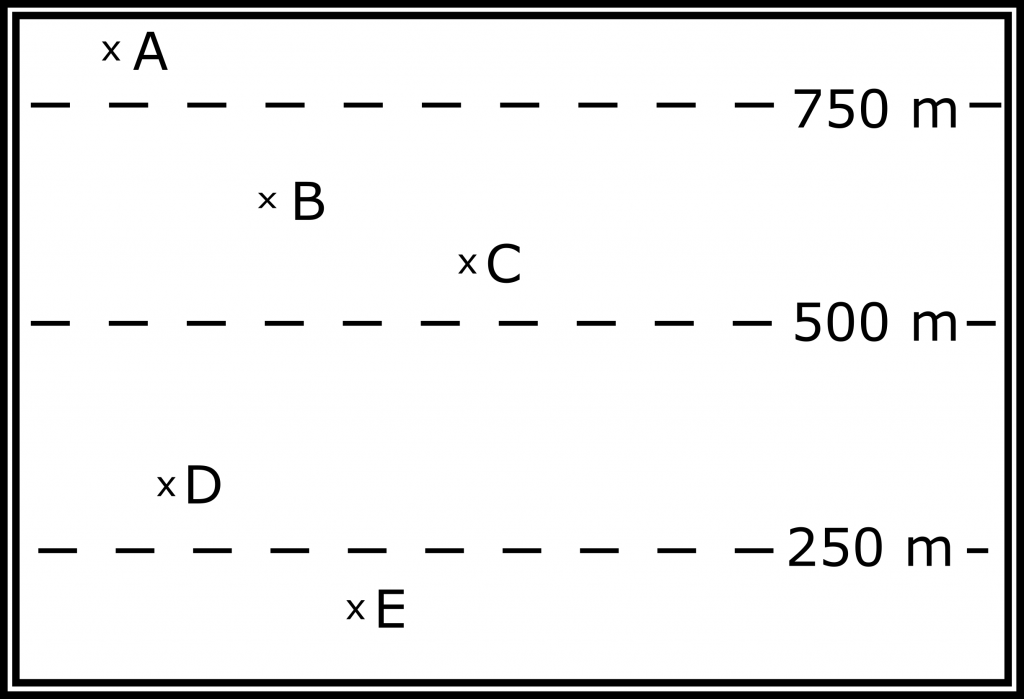
2. (5 pts) Figure 7-E4 shows five waypoints (A, B, C, D, and E) on a topographic map. Answer the following questions about these waypoints, based on your best guess estimate of the elevation of each waypoint. Note: there is technically more than one correct answer for some of these questions. Please use Occam’s razor as you answer the questions: use the simplest explanation rather than the most complicated explanation to answer the question.
a. Write your estimates for the elevation at each waypoint next to the waypoint.
b. Describe how you decided on an estimated elevation for points A and E.
c. Is the elevation of waypoint A > (greater than) or < (less than) waypoint E?
d. Is the elevation of waypoint D > or < waypoint C?
e. Is the elevation of waypoint A > or < waypoint B?
f. Is the elevation of waypoint C > or < waypoint B?
3. (10 pts) Imagine you are a geologist working for the Geological Survey of Canada. You are tasked with creating your own coastal topographic map, so you hike around a coastal area with a GPS receiver (Global Positioning System) and every so often you record your position along with the elevation in metres at that point, which results in the map below (Map 7-E5). Complete this map by adding in contour lines using a contour interval of 100 m. Draw the contour lines so that they are continuous: they will either continue to the edge of the map or form an enclosed circle. Refer to the topographic map in Figure 7-E3 for an example of contour lines you can use to help you complete this question. Your contour lines will generally fall between the GPS points on your map, so you will need to estimate many of the contour line positions. Don’t forget to add a contour line to the map legend!
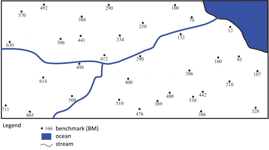
Source: Joyce M. McBeth (2019) CC BY-SA 4.0, after Brad Deline (2017) CC BY-SA 3.0 view source
The overview section 7.4.2 provides useful background to help you answer questions 4 & 5.
- (5 pts) Construct a topographic profile for the map in Figure 7-E6 from position A to A’ on the graph paper provided in Figure 7-E6 below.
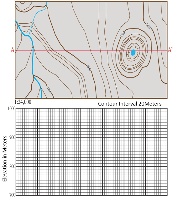
Source: Sean Lacey (2018) CC BY 4.0, after Brad Deline (2017) CC BY-SA 3.0 view source
- (3 pts) Based on the scale chosen for you for the topography (vertical axis), calculate the amount of vertical exaggeration on the topographic profile you constructed for question 4. Show your work.
Questions 6 to 16: MAP 092G095 Mt. Garibaldi Area, B.C.
For the following exercises, please refer to British Columbia Topographic Map 092G095 of the Mount Garibaldi area in southern BC. A thumbnail version of the map is shown in Figure 7-E7, a larger copy is provided at the back of this lab manual, and your TA will provide you with a full-scale version of the map in lab.
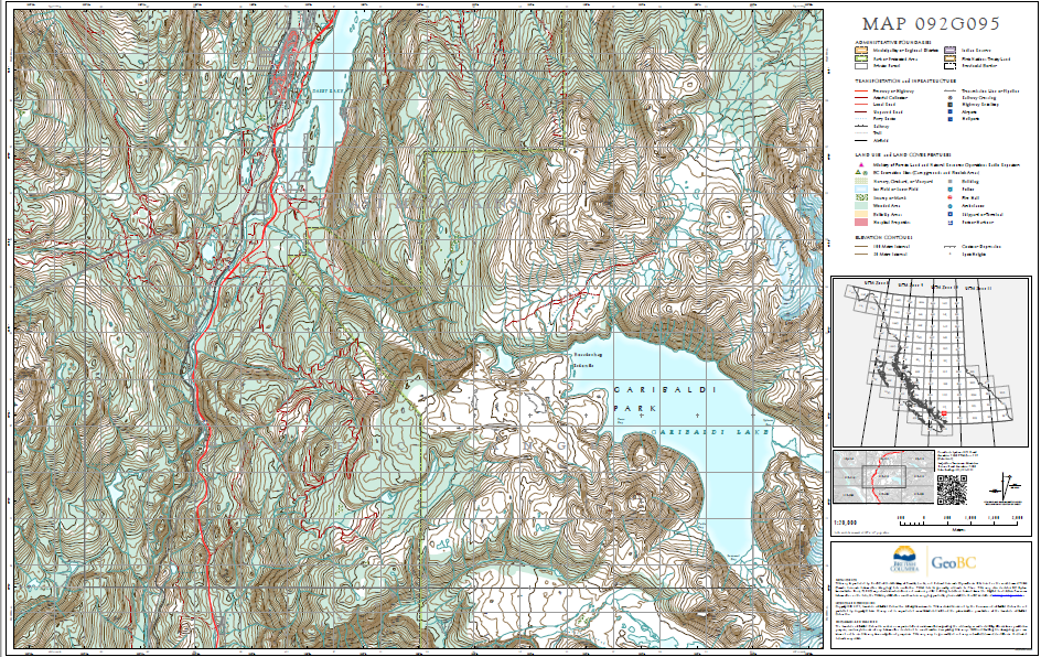
6. (1 pt) What is the ratio scale of this map?
7. (1 pt) Explain in a sentence how a ratio scale works.
8. (1 pt) Examining your map, you will see there is a black line that outlines a rectangle that takes up most of the map area. What is the latitude on the northern edge of this rectangle?
9. (1 pt) What is the longitude along the eastern edge of this rectangle?
Source: British Columbia Topographic Map 092G095, Province of British Columbia © 2016 all rights reserved view source
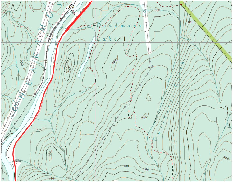
10. (1 pt) Find Deadmans Lake (it is located close to Cheakamus River and south of Daisy Lake; refer to Figure 7-E8 which is a close up from the map area). Using the surrounding contour lines, what is the approximate elevation of Deadmans Lake? Note: if you are unable to read the contours on the map, view the original map on the web or look at the large printed copy in the lab.
11. (1 pt) Garibaldi Creek is located east of Deadmans Lake (Figure 7-E8). Using the contour lines, determine the upstream direction of the creek. How were you able to come to this conclusion?
Source: British Columbia Topographic Map 092G095, Province of British Columbia © 2016 all rights reserved view source
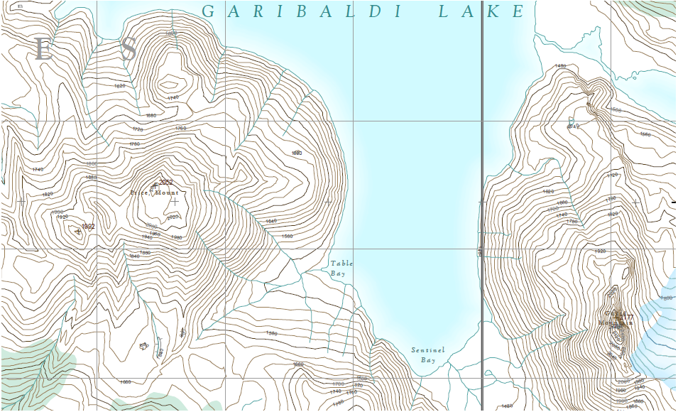
12. (1 pt) Mount Price is located next to Garibaldi Lake (just west of Table Bay, Figure 7-E9 above). Determine the height of Mount Price.
13. (1 pt) How much higher is Mount Price than Garibaldi Lake?
14. (2 pts) What is the gradient between Garibaldi Lake and Mount Price? Show your work below. Mark Figure 7-E9 with a line to indicate the distance you used in your calculation.
15. (2 pts) How would the gradient change if you measured from the peak of Guard Mountain (on the east side of the lake, across from Mount Price) to Garibaldi Lake? Explain why.
16. (1 pt) If someone decided to climb Mount Price, what would be the easiest and safest route to take? Explain why. Hint: draw a simple map or a rough cross-section sketch to help illustrate your logic.
Questions 17-19: Saskatoon Area Topographic Map
Please refer to this Saskatoon topographic map to complete the next three questions. A thumbnail version of the map is shown in Figure 7-E10, a larger copy is provided at the back of this lab manual, and your TA will provide you with a full-scale version of the map in lab.
https://openpress.usask.ca/app/uploads/sites/52/2018/08/SKtopomap_v2.pdf
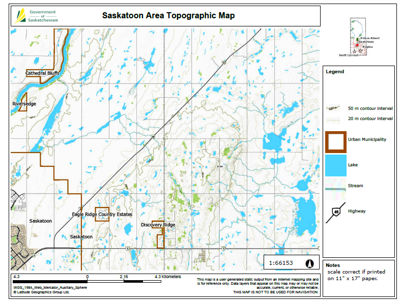
17. (2 pts) What is the ratio scale used on this map? Why would a smaller ratio scale be used for this map in comparison to the Garibaldi map?
18. (2 pts) What is the relief on this map? Give the elevation of the highest and lowest contour lines as well as the difference between them.
19. (1 pt) Contour intervals located on this map are few and far between. Why is this so?
