
Cash Flows and Cash Flow Diagrams
Cash flows are a fundamental tool in engineering economic analysis. Cash flows represent transactions in which money changes hands between two or more parties – lending $10.00 to a friend or making a payment on a car loan, for example. Representing transactions as cash flows makes it easier to keep track of the important information included in the transactions. Specifically, there are two characteristics of financial transactions that are indicated in cash flows:
- Value – the magnitude of the transaction being described. This is dependent on two factors: the amount of money or currency changing hands (a dollar value) and the direction in which the money is flowing (the orientation of the cash flow). We represent financial gains (also called receipts or income) as positive in value, and financial losses (also called disbursements or expenses) as negative in value.
- Timing – the time or period in which the cash flow occurs. Often, periods are set to coincide with interest periods, which will be discussed further in the Time Value of Money chapter. Typically, periods are in increments of months, quarters (1/4 of a year), semi-annual, or annual but other time increments may also be used.
Let’s use the example of someone lending $10.00 to a friend. We’ll assume Riley lends his friend Chris $10.00 on January 1, and Chris pays back the $10.00 on February 1. There are two transactions in this example: the initial lending on January 1, and the repayment on February 1. Each can be represented by its own cash flow. From Riley’s perspective, as the lender, the two cash flows would look like so:
| Cash Flow | Timing | Value |
| Lend $10 to Chris | January 1 | -$10.00 |
| Receive $10 from Chris | February 1 | +$10.00 |
The table in Table 1 gives a concise summary of the two cash flows involved in the example, from the lender’s perspective. But how would things change if we made the same table from Chris’s (the borrower’s) perspective?
| Cash Flow | Timing | Value |
| Receive $10 from Riley |
January 1 | +$10.00 |
| Repay $10 to Riley | February 1 | -$10.00 |
As we can see by comparing Tables 1 and 2, changing perspectives changes the signage of the cash flows. This is because when one party gives money to the other, the recipient’s total assets increase, and the donor’s assets decrease.
The previous example shows how cash flows can be used to summarize the important information in financial transactions. When conducting an analysis in a spreadsheet it is common to list cash flows in tabular format. When trying visualize or explain the financial transactions in a particular analysis, cash flows can be represented in a much simpler way – the cash flow diagram. The next section covers cash flow diagrams in detail.
Cash Flow Diagrams are simple graphical representations of financial transactions. The diagrams consist of arrows, such as in the diagram shown below.
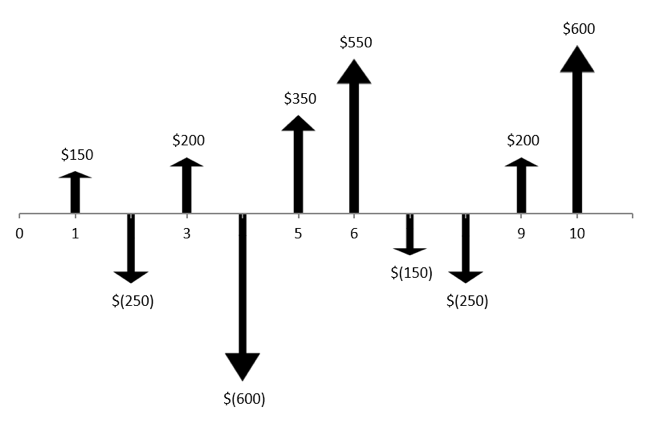
Cash flows like the ones shown in the above figure are typical. There are some basic rules for creating cash flow diagrams:
- Time is represented by a horizontal line marked with the number of periods in the analysis. The choice of time interval will reflect the project or transactions being considered.
- The horizontal position of each arrow indicates the timing of that cash flow.
- Upward arrows represent positive cash flows, also known as inflows, income, or receipts.
- Downward arrows represent negative cash flows, also known as outflows, disbursements, or expenses.
- Each arrow represents the net cash flow in that period (receipts – disbursements). There is only one cash flow arrow for each period representing this net value.
Let’s return to the previous example: Riley lending $10.00 to Chris. We can draw out the cash flows graphically as a cash flow diagram. Just like with the tabular form of the cash flows, we can represent the cash flows in two different diagrams: one from Riley’s perspective and one from Chris’s perspective. If we set January to be the first period, and February to be the second period, the two diagrams would look like so:
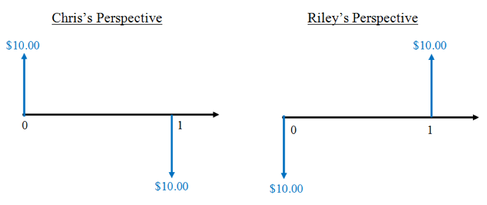
These diagrams are really just graphical representations of financial transactions. As one can see, the diagrams for Riley and Chris give the same information as the tables we showed before, but it may be less time-consuming to draw these simple diagrams than it is to write out an entire table! The movement of money is also easier to show graphically. Note that only one of the diagrams is required to represent the problem. You would simply choose to display the project from either Riley’s perspective or from Chris’s perspective.
Note that this difference in perspective does not affect the equivalence of cash flows (equivalence is covered in detail in the Time Value of Money chapter). The different perspectives affect the signs of the cash flows (i.e. positive or negative), but the net effect remains the same. In this example, both parties ended up with no net loss or gain after Riley was repaid, because no interest was charged on the loan. If Riley had charged Chris $1.00 in interest, then Riley would have earned a net profit of $1.00 and Chris would have lost $1.00 in total. The money is all accounted for, regardless of who the observer is.
End-of-Period Convention
In practice, cash flows can occur at any time within a period. However, for simplicity, we commonly assume the end-of-period convention – the assumption that all cash flows occurring within a period are moved to the end of the period. The following figure graphically demonstrates the end-of-period convention.
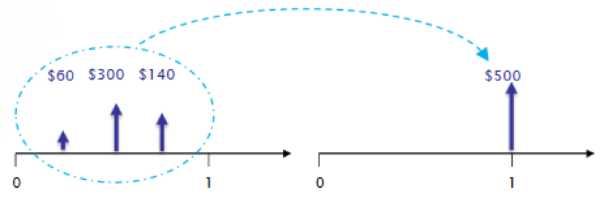
In the figure above, there are several cash flows at different times within the same period. Using the end-of-period convention, we sum these cash flows together and move them to the end of the interest period as one net cash flow.
While this assumption could introduce some discrepancies between the model and real-world results, it simplifies calculations greatly, as we will see in later chapters. The difference between the model results and real-world results are generally minor and insignificant to the analysis.
