
5.2 Basic Evaluation Methods
5.2.1 Conventional Payback Period Method
When deciding on whether to make an investment, people will often ask “How long will it take to get my money back?” This is what the payback period method allows us to determine.
The conventional payback period refers to the period of time required for the return on an investment to “repay” the sum of the original investment. Put another way, the conventional payback period of is the amount of time it takes to get back as much money as you invested. Payback period is most often calculated in years. For a one-time investment that generates a uniform series of revenues the payback period (n) is calculated as follows:

Note that n expressed in the same time units as the (recurring) revenues (e.g. years).
WARNING: this simplified equation is only applicable for a single investment with a uniform series of cash flows; more complex cash flows would require each cash flow to be considered separately.
When making decisions, people may use the payback period as a criterion by setting a benchmark time within which they want to earn their money back. If the payback period occurs before the cut-off point, the project may be accepted; otherwise, it will be rejected. In this way, the payback period can help inform investment decisions in a manner similar to the MARR.
Let’s try some examples.
Payback Period Example #1
Alex is considering purchasing a new espresso machine which can make a cup of espresso cheaper than he can buy at his local coffee shop. The machine costs $360, and he expects it to save him $60 per year. What is the conventional payback period of this purchase?
Since this example involves uniform cash flows, we can use the simplified payback period equation.
Initial investment = $360
Revenues per time period = $60/year

The conventional payback period of Alex’s new espresso machine is 6 years.
Payback Period Example #2
Brandon is considering purchasing a similar espresso machine for $375. However, Brandon is a first year engineering student, and expects that his field of study will impact his coffee consumption. If the new machine saves him $75 for each of his first three years, $100 during his fourth (and final) year of school, and $50 per year after he has graduated, what is the conventional payback period of this purchase?
Solution
Unlike the previous example, we are not dealing with a uniform series of cash flows in this example, so we cannot use our simplified equation. We solve it instead by creating a table showing cash outflow and inflows from Brandon’s perspective:
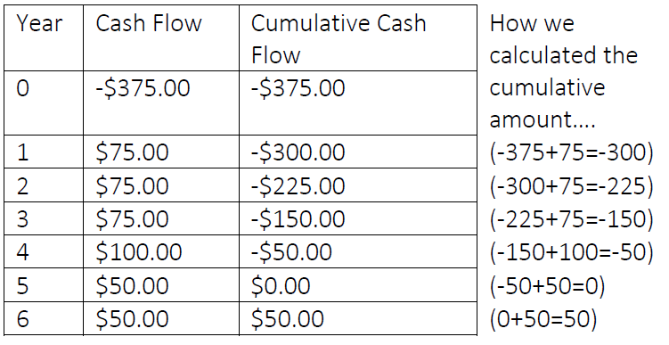
By looking at the cumulative cash flows, we can see that the initial investment is earned back at the end of year 5. At this point, the cash outflow and inflows were equal. Therefore, the conventional payback period in this scenario is 5 years.
Sometimes, like in these two examples, the payback period is easy to see because they give a cumulative cash flow of exactly $0 at the end of one of the periods.
This is not true of all cases, however. Sometimes, the cash flows will equal zero part way through a year (or other time period), so the payback period will not be a whole number. In these cases, we typically assume that the cash flows occur continuously throughout the time period (i.e. not just in lump sums at the end of each period). For example, if a project brings in $365 per year, we assume that it makes $1 per day. This allows us to use linear interpolation to estimate where the payback point occurs within the time period.
Let’s look at an example that requires linear interpolation.
Payback Period Example #3
Carla is another first year engineering student, with coffee drinking habits very similar to Brandon from Example #2. She purchases the same espresso machine as Brandon, but finds it on sale for $345. If she saves the same annual amounts as Brandon, what is the conventional payback period of her purchase?
Solution
Let’s look at the cash outflows from Carla’s perspective:
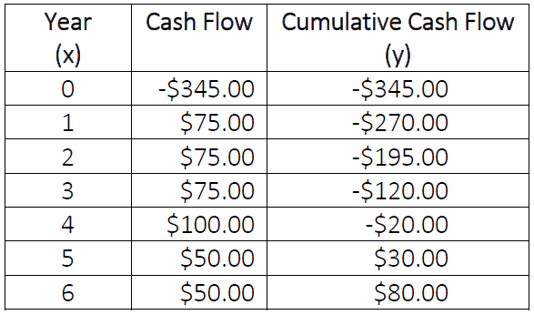
Here we see that we cannot determine the exact payback period by just looking at the cash flows because Carla’s cumulative cash flow is not exactly zero at the end of any year. We can see, however, that the cumulative cash flow is negative at the end of year 4, but positive at the end of year 5. This means that the payback period must have occurred sometime between the 4th and 5th years. We can approximate the actual time by using linear interpolation. Linear interpolation is a reasonable method in this case, because we can assume that the cash flows reflect small amounts saved each day on cups of espresso not purchased at a coffee shop.
Since we know the payback must occur between years 4 and 5, we use those as our known points. Setting years as our x-values and cumulative cash flow as our y-values, we have the two points:
(x0, y0) = (4,-$20)
(x1, y1) = (5, $30)
We now interpolate between these points to find the value of x for which y = $0. Using this information, we solve for x:


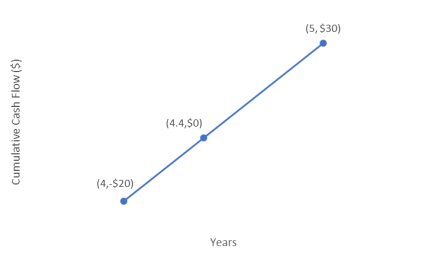
You can see in the diagram above how linear interpolation finds the point at which our cash flows are equal to zero.
Therefore, the conventional payback period for this project is 4.4 years.
Gut check: Is this reasonable? Carla paid less than Brandon, so her payback period should be less than his. Her payback period of 4.4 years is shorter than Brandon’s payback period of 5 years, so this answer is reasonable.
Advantages & Drawbacks of the Conventional Payback Period Method
| Advantages | Disadvantages |
|
|
ADVANTAGES
- Easily understood: Investors often want to know how long it will take to get their money back if they choose to invest. The payback period gives this information and can be understood regardless of academic or technical background.
- Widely used: Members of many industries use and understand this concept, allowing for straightforward communication between parties regarding investment opportunities.
- Favours liquidity: By choosing projects with shorter payback periods, a company quickly earns back the nominal value of its investment, and can invest in other projects sooner.
- Effectively measures investment risk: The project with a shortest payback period typically has less risk than with the project with longer payback period. (Boundless Finance)
DRAWBACKS
- No consideration of TVM: Since the conventional payback period method only uses the nominal values of future cash flows, it overstates the values of those cash flows because it does not account for the effect of time on their value, as discussed in Chapter 3. This becomes particularly significant for projects involving high interest rates or long time periods. For this reason, it is generally recommended that this method not be the sole criterion for decision making.
- Ignores long-term cash flows: This method does not consider any cash flows after the payback period. For example, many long-term construction projects require site cleanup costs or disposal costs after a project is finished. Also, any revenues obtained after the payback period are not considered, despite the fact that they may be substantial. The conventional payback period analysis ignores both of these factors because they occur after the project’s revenues have “paid off” the initial expenditure.
- Ignores project risk: The expected future revenues or expenses of the project used in the calculations are considered certain, and no analysis of potential risks to the project is considered.
- Arbitrary cut-off point: The conventional payback method forces the decision maker to set a strict payback point. However, there is no real reason to define a specific payback period unless there are known events that will occur beyond that period which would require you to be paid back. For example, if you know your company will need a large amount of capital available in 4 years to expand its head office, then it might make sense to expect a payback period of less than 4 years for any major projects.
- Biased toward short term projects: By emphasizing quick payback, this method downplays the importance of long-term planning.
5.2.2 Net Present Value (NPV) Analysis
The net present value (NPV) method is one of the simplest and most reliable ways to decide whether or not to undertake a project or investment. The strength of this method is its consideration of the time value of money (covered in Chapter 3).
The NPV is the sum of the present values of all costs and revenues associated with the project.
NPV is calculated using the following formula:

Notice that that equation is the present value formula, but summing multiple cash flows.
The net present value of an investment or project can be understood as the value that you could receive today that would be economically equivalent to undertaking the project. That is, accepting a $100 bill today would be economically equivalent to undertaking a project whose NPV was $100.
By calculating the NPV, we can determine whether a project is economically profitable. If the NPV is a positive number, then the project is profitable. If the NPV is a negative number, then the opposite is true: the project is not profitable and should not be accepted (if profit is the only goal of the project). If the NPV is at least zero, then the project meets the specified MARR. Note that in reality, a project may be accepted or rejected based on other factors, such as public image.
Sometimes, you may have the opportunity to choose from several different projects, but can only choose one and must reject all others. In this situation, we say the projects are mutually exclusive. The NPV method can help us decide which project to accept. When given multiple mutually exclusive projects, the one with the highest NPV should be accepted. Note, however, that if all the projects have negative NPVs, we should likely still reject all of them.
To calculate the NPV of a project, we need some initial information:
- The discount rate of the project. This rate is usually the company’s MARR.
- The expected timing and amounts of all cash flows of the project. More accurate estimates of these values will give a more accurate NPV.
To refresh your concept of present value and the time value of money, consider the following example:
Erica sees that a local lottery is advertising a $1.5 million dollar prize, so she buys a ticket, and ends up winning. After winning, the lottery company contacts her and informs her that her $1.5 million dollar prize will be awarded over the course of 10 years, with a $150,000 payment each year beginning today, rather than as a lump sum today. Erica is overjoyed at having won, so she accepts these terms without considering the time value of money. If her local bank offers an interest rate of 5%, how much more preferable would the lump sum payment have been?
Since a dollar today is worth more than a dollar tomorrow, it will be better for Erica to have her money up front. To see this difference, we must find the present value of the ten-year series of payments, and compare it to the $1.5 million lump sum.
We will show the present value calculations explicitly for the first three payments, and then show the remainder of the process in a table. Note that the first payment is received immediately, and so its present value will still be equal to $150,000.


| Year of Cash Flow | Present Value |
| 0 | $150,000.00 |
| 1 | $142,857.14 |
| 2 | $136,054.42 |
| 3 | $129,575.64 |
| 4 | $123,405.37 |
| 5 | $117,528.92 |
| 6 | $111,932.31 |
| 7 | $106,602.20 |
| 8 | $101,525.90 |
| 9 | $96,691.34 |
| Sum (NPV) | $1,216,173.25 |
Thus, the NPV of a project is $1,216,173.25. Since the NPV of a lump sum payment is $1.5 million, the difference is:
$1,500,000.00 – $1,216,173.25 = $283,826.75
So, although Erica will still receive $1.5 million (the nominal amount), the economic (real) value of her prize is $283,826.75 less because it is paid over 10 years.
The Do-Nothing Alternative
In many cases, investment is not required, and the do-nothing alternative exists. The term “do-nothing alternative” can mean two distinct things:
A) Do not invest in any alternatives and do nothing; or,
B) Do not invest in any alternatives and continue as is.
In Case A, all cash flows are zero. There are no investments, revenues, or costs. This simply means that if we are presented with several projects to choose from and none of them are desirable, we can decline all of the options. However, in Case B (also known as the status quo), no new investment is made and the costs and revenues are merely those being incurred under current operations.
Examples do-nothing alternatives include:
- You are considering starting a business, and have estimated your costs and revenues. If the NPV is negative, you should not start the business. This option of doing nothing results in neither a financial gain nor a financial loss (Case A).
- A corporation considering acquiring a competing business. If the acquisition appears to be unprofitable, then the corporation would not pursue the acquisition and continue operating as is (Case B).
However, the do-nothing alternative is not always available. Some examples of situations in which the do-nothing alternative is not available include:
- A company deciding to replace something vital to its business, such as a Coca-Cola bottling plant replacing its bottle-filling machines as they wear out.
- A car dealership owner deciding what vehicle models to order and sell from his supplier.
- A growing city upgrading its sewer system and wastewater treatment plant.
In these cases, the decision maker cannot choose the do-nothing alternative. Put another way, they must choose at least one of the options being considered. If the bottling plant does not replace its equipment as it wears out, eventually the machines will no longer be functional, and the business will have to shut down production. Similarly, if the car dealership does not order new vehicles as it sells the vehicles in its inventory, it will run out vehicles and cease to operate. If the city does not expand its sewage management infrastructure… you get the idea.
When the do-nothing alternative is not available, economic analyses only need to compare investment/purchase/project opportunities against each other; for example, the bottling plant simply needs to select which bottle-filling machine is most profitable (or least expensive).
Below is a list of pros and cons of the NPV method.
| Advantages | Drawbacks |
|
|
ADVANTAGES
- Easily understood: Investors want to know which potential investments will provide them with the most economic value. The NPV method gives this information and can be understood regardless of academic or technical background (Boundless Finance).
- Widely used: Members of many industries use and understand this method, allowing for straightforward communication between parties regarding investment opportunities.
- Favours wealth maximization: The NPV method measures the size of the profits to be made, unlike some methods which only measure the relative profitability of the project.
For example, suppose you have two mutually exclusive projects: A and B. The project details are given in a table.
| Project | Initial Cash Outlay ($) | NPV of Entire Project ($) |
| A | 1 | 10 |
| B | 100 | 500 |
In this case, some other methods, such as the IRR method, would declare that project A is the better option because it has a higher return on investment. However, if the projects are mutually exclusive and you cannot repeat the same project it is clear from the NPV method that project B should be chosen because it maximizes profits. In the NPV method, we do not care about the efficiency of investments – only wealth maximization.
- Easily understood: The NPV method is easy to understand because it answers a simple question: what should I invest in to get the highest profits for myself or my company? Net present value analyses are easy to explain to audiences who may not know much about the mathematics of finance. This is very important in industry, where investment decisions often require approval from a manager or board of directors who are not familiar with the projects themselves.
- Considers TVM: By discounting all future cash flows and comparing them in a common timeframe, the net present value method allows us to calculate the true economic value of cash flows in a project or investment. This, of course, leads to better financial decisions than if the time value of money were ignored, as it is in analysis methods such as the payback period method.
- Easily adjusted by discount rate: NPV is very sensitive to the discount rate used in the calculation. This means that if you are skeptical of a project’s viability, or uncertain about the value and timing of the cash flows, you can raise the interest rate to see if the project is still profitable.
DRAWBACKS
- Highly sensitive to discount rate: NPV analysis is essentially just discounting cash flows, which makes it highly sensitive to the discount rate chosen. This means that choosing the correct discount rate is important in NPV analysis. However, it is often difficult to know exactly what discount rate is appropriate, so assumptions must be made when choosing a rate. Basing the discount rate on insufficient information and large assumptions increases the error in NPV calculations.
- Requires future cash flow estimates: NPV analysis requires reasonable estimates of all future cash flows – both their timing and their amounts. Often, accurate estimates of future cash flows are difficult to obtain. For example, when deciding whether to purchase a new piece of equipment, it may be hard to predict annual maintenance costs or cost savings. The more uncertain we are about the revenues and costs of the investment, the more error in the NPV calculation.
- Ignores opportunity cost: “Furthermore, the NPV is only useful for comparing projects at the same time; it does not fully build in opportunity cost. For example, the day after the company makes a decision about which investment to undertake based on NPV, it may discover there is a new option that offers a superior NPV. Thus, investors don’t simply pick the option with the highest NPV; they may pass on all options because they think another, better, option may come along in the future. NPV does not build in the opportunity cost of not having the capital to spend on future investment options.”(Boundless Finance)
- Requires identical project duration: The only way to compare projects of different durations using the NPV method is to analyze them over a period that is equal to the least common multiple of the individual projects’ periods.
When the do-nothing alternative is available, it can be considered in one of two ways:
A) By evaluating it as an explicit option like any other project, but with all revenues and costs equal to zero
or
B) By measuring all the other alternatives against the do-nothing alternative, and subtracting its cash flows from the option being considered.
NPV Example
You own a ceramics manufacturing company. The ovens your plant currently uses are expected to last another 8 years. You are considering replacing your ovens with a newer, more efficient model that saves heating costs. You estimate that outfitting your plant with the new ovens would cost $3 million, the ovens would last 8 years, and the move would save the company $400 000 per year, starting next year. If your company’s MARR is 4%, is the project worth undertaking?
Solution
In order to determine whether the project is worth undertaking, we can simply determine the net present value of the cash flows.
𝑁 = 8 years
𝐴 = $400 000
𝑖 = 4% = 0.04

Since the NPV of the project is negative, the project should be rejected.
5.2.3 Annual Equivalent Value (AEV) Analysis
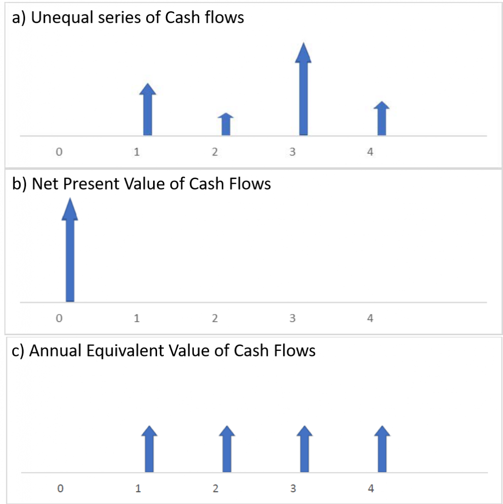
Rather than considering how much a project will earn us overall using the net present value (NPV) method, we may prefer to know how much it will earn us over time. For this, we use the annual equivalent value (AEV) method, which converts the NPV of our project into an economically equivalent, uniform series of cash flows. This allows us to visualize how much our project will earn us (or cost us) each year. For example, this may be useful when considering two projects with an equivalent NPV, but different durations; the shorter project earns money in a shorter time frame, and therefore would have a higher AEV.
To visualize this process, consider the following three cash flow diagrams. All of these diagrams are economically equivalent; that is, they all have the same NPV. The first diagram shows an unequal series of cash flows, like you might receive from a 4-year project. The second diagram converts these cash flows into a single cash flow in Year 0, which is the NPV of the project. The final diagram converts this NPV to an annual equivalent value, so that each year we see an equal revenue being produced. All of these have the same NPV.
The formula to convert a project’s NPV to an AEV is:

Notice that this is an adaptation of the payment-from-present-value formula introduced in Chapter 3. Since AEV analysis is an adaptation of NPV analysis, it has many of the same advantages. In particular, it accounts for the TVM and emphasizes wealth maximization, unlike the conventional payback period method.
Advantages & Drawbacks of the Annual Equivalent Value (AEV) Method
| Advantages | Drawbacks |
|
|
ADVANTAGES
- Easily understood: An investor may wish to know how much they will earn from a project on an annual basis. The concept of a consistent annual return on investment can be understood regardless of academic or technical background.
- Favours wealth maximization: As with NPV analysis, AEV analysis measures the size of potential profits rather than their relative profitability. This means that it will favour projects which maximize wealth.
- Considers TVM: The discount rate applied in AEV analysis (usually MARR) allows for the method to account for the time value of money.
- Easily adjusted by discount rate: As with NPV analysis, AEV analysis can be tested at multiple discount rates in order to evaluate its likely profits.
DRAWBACKS
- Highly sensitive to discount rate: Since this method is so easily adjustable by the discount rate, it is also very sensitive to that rate, and a slightly unrealistic rate can produce misleading results.
- Requires future cash flow estimates: AEV analysis requires accurate estimates of the timing and amount of future cash flows; the more inaccurate the estimates, the more inaccurate the AEV will be.
AEV Example
You work for a potash mine that plans to temporarily expand its processing facilities for a cost of $2,000,000. This expansion will increase profits by an estimated $740 000 annually. Maintaining the new facilities will cost $20,000 during the first year of operations, and this cost will increase by $1500 each year as the equipment deteriorates. If the expansion is put in place for a period of 4 years and the mine applies an MARR of 10%, what is the annual equivalent value?
Solution
1 – Begin by finding the NPV of the initial cost (1), annual profits (2), and annual operating costs (3). Notice that the increased profits represent a linear series, while the cost of operations is a gradient series.
i = 10% = 0.1
N = 4 years
NPV1 = -$2,000,000


2 – Sum the NPVs to find the total net present value of the project.
NPV = NPV1 +NPV2 +NPV3 = -$2,000,000 + $2,345,700.43 -$69,964.48
NPV = $275,735.95
3 – Convert this NPV to an annual equivalent value (AEV)

The Annual Equivalent Value of the expansion is $86,986.64.
5.2.4 Capital Recovery Cost (CRC) Analysis
The capital recovery cost (CRC) method is useful when evaluating an investment that can be salvaged or resold at the end of its project duration. CRC analysis adapts AEV analysis by considering the initial price and future salvage value of the investment, and combining them as an annual equivalent cost. This means that the CRC is an estimate of the average cost a company would pay per year to operate a project, when only the initial cost (P) and salvage value (S) are considered:

You should notice that the first term of the equation, which accounts for the initial price of the investment is derived from the annual given present value equation. Similarly, the second term dealing with the project’s salvage value is derived from the equation for annual given future value. Both of these equations are explained in Chapter 3.
The value of this method is to show a company how much it must earn from an investment per year in order for it to be profitable. If a project is expected to generate less annual revenue than its CRC each year, then it should be rejected. Note that the formula for CRC incorporates the company’s MARR as its discount rate, so that a project which earns more than its CRC overcomes the company’s expectations for opportunity cost, inflation, cost of capital, and risk. It should also be noted that in some cases CRC can be an insufficient basis for the financial strength of a project, since it does not consider any ongoing costs associated with the project beyond its initial price.
Advantages & Drawbacks of the Capital Recovery Cost (CRC) Method
| Advantages | Drawbacks |
|
|
ADVANTAGES
- Favours wealth maximization: As with NPV and AEV analyses, CRC analysis measures the size of potential profits rather than their relative profitability. This means that it will favour projects which maximize wealth.
- Considers TVM: The discount rate applied in CRC analysis (usually MARR) allows for the method to account for the time value of money.
- Easily adjusted by discount rate: As with NPV and AEV analyses, CRC analysis can be tested at multiple discount rates in order to evaluate its likely profits.
DRAWBACKS
- Highly sensitive to discount rate: Since this method is so easily adjustable by the discount rate, it is also very sensitive to that rate, and a slightly unrealistic rate can produce misleading results.
- Requires salvage value estimate: CRC analysis requires an accurate estimate of the salvage value at the end of a project, which may be difficult to predict.
CRC Example
Noah’s company buys him a new pickup truck for conducting field surveys. The truck costs $32 000, and after 5 years of use the company plans to resell it for $24,000. If Noah’s company uses an MARR of 8%, what is the Capital Recovery Cost (CRC) of this investment?
Solution
P = $32,000
S = $24,000
i = 8% = 0.08
N = 5 years
1 – Apply the standard capital recovery cost formula


The capital recovery cost of the new truck is $3923.66
Remember that this value is equivalent to the annual cost of owning the truck, and this investment must generate over $3923.66 per year for it to be a worthwhile investment.
5.2.5 Internal Rate of Return (IRR) Method
As discussed at the beginning of this chapter, the rate of return for a project is a percentage showing the total profits divided by the investment cost. This concept allowed us to consider the minimum acceptable rate of return (MARR), which could be used as a discount rate when determining the viability of a project. In order to compare the return on our project directly to our MARR, we can calculate the internal rate of return (IRR).
The IRR is defined as the discount rate (usually annual) that gives a project a net present value of zero. In more specific terms, the IRR of an investment is the discount rate at which the net present value of the costs (negative cash flows) of the investment equals the net present value of the benefits (positive cash flows) of the investment. The term “internal” refers to the fact that its calculation does not incorporate environmental factors (e.g., the interest rate or inflation).
IRR calculations are commonly used to evaluate the desirability of investments or projects. If a project’s IRR exceeds a company’s MARR, then it is worth investment. The higher its IRR, the more desirable it is to undertake the project. Why? Let’s do a couple of thought experiments.
- There are two projects, each of which costs $1000. Project A returns $1400 after two years, and Project B returns $1500 after two years. Which of these would you prefer?
- There are two projects, each of which return $1600 after two years. Project C costs $1400 up front, and Project D costs $1500 up front. Which of these would you prefer?
In these scenarios, it is fairly straightforward to determine which project is economically preferable. Now, let’s use these questions to show how IRR can be used to make decisions.
1 – There are two projects, each of which costs $1000. Project A returns $1400 after two years, and Project B returns $1500 after two years. Which of these has a higher IRR?
We will calculate the internal rate of return for each by setting our NPV equation equal to zero:

|

|


We see that Project B has a higher IRR than Project A because it produces a greater return for the same initial cost, and thus would be the better investment.
2 – There are two projects, each of which return $1600 after two years. Project C costs $1400 up front, and Project D costs $1500 up front. Which of these has a higher IRR?

|

|


We see that Project C has a higher IRR than Project D because it produces the same return for a lower initial cost, and thus would be the better investment. Notice that both of these rates of return are fairly low; if you had a MARR of 8%, you would choose to reject both of these projects.
As we can see from these examples, the project with the highest IRR should be considered the best and undertaken first. A firm (or individual) should, in theory, undertake all projects or investments available with IRRs that exceed their MARR. That is, if the IRR is greater than the MARR, accept the project; if the IRR is less than the MARR, reject the project. In practice, a company might not accept all projects with an IRR exceeding the MARR because they may not have enough money or resources available to do so.
You may wonder: are decisions based on IRR similar to decisions based on NPV? When a project’s IRR is equal to its MARR, it will have an NPV of zero. If we approve projects with an IRR greater than our MARR, then we are approving all projects with positive NPVs; this means that the NPV and IRR methods will agree on whether an individual project should be accepted. However, determining whether a project yields a profit is different from determining which projects are more profitable. When evaluating several mutually exclusive projects, the IRR method may favour a different project than the NPV method. This is because IRR maximizes investment efficiency (money earned per dollar spent), whereas the NPV method maximizes wealth (net money earned). So, the evaluation method you select will depend on your investment priorities.
Calculating the IRR
Given a set of cash flows occurring at different times during a project, the internal rate of return can be found by setting the net present value equation equal to zero and solving for ‘i’. As always, the time units must be consistent for each cash flow (e.g. weeks, months, years).
For example, if an investment may be given by the following sequence of cash flows:
Step 1: Write the NPV equation for this series of cash flows, and set it equal to zero.


Step 2: Solve for “i”.
In this case, the answer is 14.3%. You may have noticed that this equation is not easy (okay, let’s admit it: basically impossible) to solve by hand. So, how did we arrive at this answer?
5.2.5.1 Methods for Calculating the IRR
Let’s look at three methods for calculating a project’s IRR:
- Direct solution
- Trial and error
- Graphical solution
Method 1: Direct Solution
The direct solution method is essentially only practical in two cases: A) when the project has only one cash outflow and one cash inflow, and B) when the project has one cash outflow and a return for two periods.
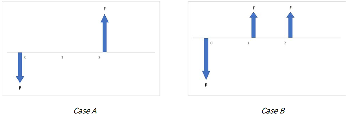
Case A
In this case, direct solution is fairly straightforward using the net present value formula, We will show this in the two examples below.
IRR Example 1
Assume you spend $2000 today, and receive a return of $3500 in 4 years. What is the internal rate of return for this investment?
Solution
Since this is a problem with only one cash inflow and one cash outflow, we can isolate the internal rate of return, i, and solve for its value using our known information (the cash flow amounts and timing) by setting the NPV equation equal to zero.
P = -$2000
F = $3500
N = 4 years


![i = \sqrt[4]{1.75} - 1](https://openpress.usask.ca/app/uploads/quicklatex/quicklatex.com-96f519cf09834b79d75fb34a67030b1e_l3.png "Rendered by QuickLaTeX.com")

So the IRR for this project is 15%.
IRR Example #2
Assume you spend $2000 today, and you receive returns of $1300 after 1 year and an additional $1500 after 2 years. What is the rate of return for this investment?
Solution
This problem involves three cash flows instead of two, but may still be solved using the direct solution method.
Step 1: Write out the project’s NPV as a series of cash flows, and set equal to zero:

Step 2: Solve for i. In this case, we cannot isolate i because of the exponent of the rightmost term. However, we can make this easier by using a substitution:
![\text{let x} = \frac{1}{1+i} So: [latex]NPV = 0 = -2000 +1300x + 500x^2](https://openpress.usask.ca/app/uploads/quicklatex/quicklatex.com-2fd42237bcecce3ebac718dfe24ca118_l3.png "Rendered by QuickLaTeX.com")
Now we can solve for x using the quadratic equation.


Now that we have the values of x, we can use them to calculate i.

As you can see, we obtain two possible answers for i. So which one is correct? In this case, we can assume that the IRR is 25%, since an IRR of -160% would imply that the project had cost more than 100% of the initial investment price; this is impossible, since all subsequent cash flows were positive. So the IRR is 25%. However, this problem illustrates a shortcoming of the IRR method: there are many situations where mathematical operations will yield two or more possible values for the IRR.
Method 2: Trial-and-Error
The trial and error method is the process of “guessing” the IRR until the correct value is found. The steps are as follows:
- Make an initial guess for the internal rate of return (IRR). Calculate the project’s NPV using that guess.
- If the calculated NPV is positive, increase your guess for the IRR and calculate the NPV again. If the NPV is negative, decrease your guess for the IRR and calculate the NPV again.
- Repeat steps 1 and 2 to continually bring the NPV closer to zero. As the NPV approaches zero, the IRR will approach its true value.
The trial-and-error method can be very tedious to do by hand or with a basic calculator. It is relatively easy to do with a spreadsheet or more advanced calculator.
Method 3: Graphical Solution
The graphical solution method is similar to the trial and error method. Both calculate multiple values of the NPV by varying the discount rate (i). It can also be done easily on a spreadsheet/graphing program. For this method, we select a reasonable range for the rate of return for the project, and then calculate the NPV for these rates. When we graph these data points, they will generate a continuous line graph. And since we know that the IRR of a project is the rate of return which results in a NPV of zero, we look for the point on our line where NPV = 0. This will give the IRR for the project.
Example
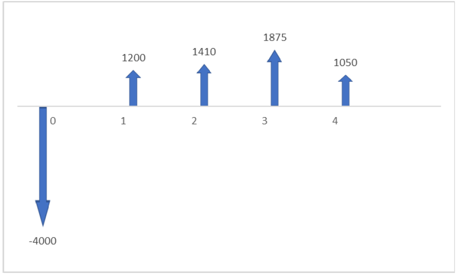
Suppose you expect the following series of cash flows from a project and want to determine the IRR.
Consider the NPV equation for this series of cash flows:

Solving this equation using Method 1 would be very complex and time consuming. Let’s try Method 2.
Step 1: Make a guess for the internal rate of return. As a starting point we will guess 5%
Step 2: Calculate the NPV of the project using a discount rate of 5%.
This will generate an answer of $985.61. Since this value is significantly positive we will increase our guess for IRR substantially to 10% and try again. If our answer had been negative, we would have decreased our guess.
Iterate this process several times, increasing and decreasing your guess each time as necessary. A series of guesses might look like this:
| IRR Guess | NPV | Result |
| 5% | $985.61 | Increase Guess |
| 10% | -$91.76 | Decrease Guess |
| 9% | $107.51 | Increase Guess |
| 9.5% | $6.94 | Increase Guess |
| 9.55% | -$3.02 | Decrease Guess |
| 9.54% | -$1.02 | Decrease Guess |
| 9.53% | $0.96 | Increase Guess |
We can see that the IRR for the project is approximately 9.53%, since it reduces the NPV of the project to nearly zero. The exact IRR must lie between 9.53% and 9.54%, but further precision would require many more iterations. If we wished, we could iterate further, and we would find that the exact IRR for the project is 9.53482776347522%. However, this level of precision is not useful for our purposes.
To check our answer, let’s solve the question again using Method 3.
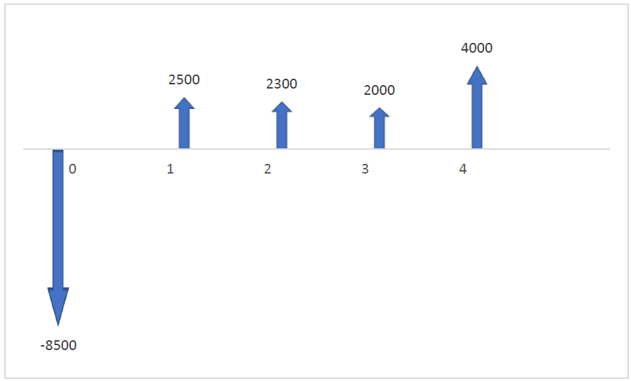
Select a range of possible values which might contain the IRR. For example, suppose we looked at values between 12% and 16%. If the IRR is in this range (i.e. NPV is equal to zero at one point between these two values), then the NPVs of 12% and 16% will have opposite signs. If we calculate NPV for these two values using the equation applied in Method 2, we get the following results:
NPV(12%) = -$468.68
NPV(16%) = -$1145.07
Since both of these results are negative, we know that the IRR does not occur in this range. If we guess a lower discount rate, like 8%, we get an NPV of $314.48. Since this is a positive value, we know that the IRR must be between 8% and 12%, so we can search for it in this range.
Calculate the NPV of the project for possible IRRs within the range, using the same NPV equation as was used with Method 2. For this example, we will evaluate NPV at 0.5% increments. This will produce the following results:
| IRR | NPV |
| 8.0% | $314.48 |
| 8.5% | $210.01 |
| 9.0% | $107.51 |
| 9.5% | $6.94 |
| 10.0% | -$91.76 |
| 10.5% | -$188.63 |
| 11.0% | -$283.71 |
| 11.5% | -$377.05 |
| 12.0% | -$468.68 |
Graph the pairs of IRR and NPV values, and find the intercept where NPV is equal to zero: this is the IRR of the project.
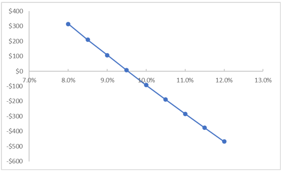
We can see that the x-axis intercept of this graph (where NPV=0) is slightly greater than 9.5%; if we were to measure it exactly, we would see that it represents an IRR of 9.53%, the same answer we obtained using the trial and error method.
Advantages & Drawbacks of the Internal Rate of Return (IRR) Method
| Advantages | Drawbacks |
|
|
ADVANTAGES
- Easily understood: Investors will often be interested in knowing the rate of return on a project. Projects with the highest IRRs should be preferred. This makes the consideration process straightforward in a way which is clear and relatable to all decision makers for a project.
- Widely used: The IRR method is commonly used in industry, and will be familiar to most individuals responsible for approving projects.
- Favours efficient investments: Since IRR is a rate percentage, it is an indicator of the efficiency, quality, or yield of an investment. This is in contrast with the NPV and AEV methods, which are indicators of the value or magnitude of an investment. Higher IRRs indicate higher profits per dollar invested.
DRAWBACKS
- Cannot compare mutually exclusive projects: IRR should not be used to rate mutually exclusive projects, but only to decide whether a single project is worth investing in. In cases where one project has a higher initial investment than a second mutually exclusive project, the first project may have a lower IRR (expected return), but a higher NPV (increase in shareholders’ wealth) and should thus be accepted over the second project (assuming no capital constraints).
- Requires future cash flow estimates: IRR analysis requires accurate estimates of the timing and amount of future cash flows; the more inaccurate the estimates, the more inaccurate the calculated IRR will be.
- Requires identical project durations: Since IRR does not consider cost of capital, it should not be used to compare projects with different durations. Modified Internal Rate of Return (MIRR) does consider cost of capital by applying an MARR, and provides a better indication of a project’s efficiency in contributing to the firm’s discounted cash flow.
- May produce multiple values: In the case of positive cash flows followed by negative ones and then by positive ones, the IRR may have multiple values.
5.2.6 MIRR: An Alternative to the IRR Method
Although the IRR method remains widely used, some issues with the method led to the development of a modified, alternative rate of return method. To understand this alternative method, we should first consider two of the key drawbacks to IRR calculations: a) multiple IRRs, and b) reinvestment assumptions.
a) Multiple IRRs
In Figure 5.4 (Method 3) the graph plotting the NPV in relation to the IRR of the project yielded a straight linear function, so there was only one point, or intercept where the NPV was equal to zero, and thus only one IRR value. However, sometimes the relationship between a project’s NPV and IRR is non-linear, and there are multiple intercepts representing potential IRR values. We can see an example of this in the NPV-IRR graph below (Figure 5.5), where potential IRR values appear at both 8% and 92%.
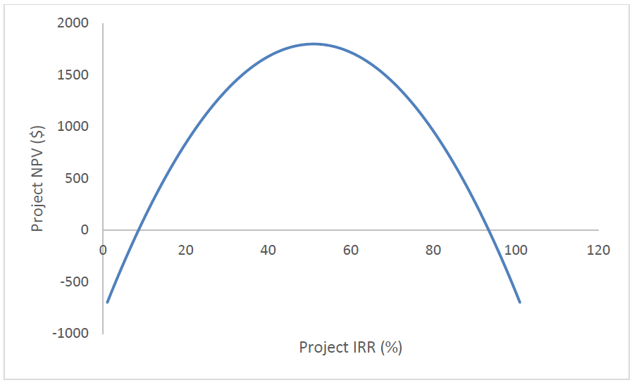
This type of result occurs when the cash flows relating to a project alternate between positive and negative more than once over the time period being studied. The more times these values alternate, the more potential IRR values will be generated, and the more confusing it can become to determine the true IRR of a project.
b) Reinvestment of Cash Flows
The second major drawback of the IRR method is that it assumes that any revenues produced by the project can be reinvested at a rate equal to the project’s IRR. For example, assume we have a 10-year project with a calculated IRR of 25% and in Year 2, the project produced a revenue of $1000. In order for the project to actually have an IRR of 25%, this $1000 revenue would need to be reinvested in a new project that also had a 25% rate of return. However, suppose that the next best project available to us only has an IRR of 15%. If we invest our $1000 revenue in this less lucrative project, then our original project will have an effective rate of return lower than 25%, and the IRR method will have overestimated its value.
We can deduce that this must be a common problem with the IRR method because we will probably invest in the most profitable project first, so any subsequent projects we can reinvest in are very likely to have lower IRRs. As a result, we will likely overestimate the benefit of our first project.
This brings us to the Modified Internal Rate of Return…
The modified internal rate of return (MIRR) method addresses both of these problems. First, it groups together all negative and positive cash flows to eliminate the possibility of multiple IRRs. Second, it assumes that all revenues are reinvested at your MARR rather than at the IRR of the project, which prevents overestimation of the IRR due to unrealistic reinvestment assumptions.
There are three steps to finding the MIRR of a project:
- Convert all negative cash flows over the project duration to a single negative cash flow at the start of the project using the NPV formula. Use your MARR as the discount rate.
- Convert all positive cash flows over the project duration to a single positive cash flow at the end of the project using the future value formula. Again, use your MARR as the discount rate.
- Using the present value equation, substitute the negative cash flow as the present value (P), and the positive cash flow as the future value (F), and solve for the discount rate (i). This is the rate which makes the positive and negative cash flows equal, and thus is the MIRR of your project.
The MIRR is evaluated in the same way as an IRR: if the MIRR exceeds your MARR, then the project is a worthwhile investment; if it is less than your MARR, then it isn’t a worthwhile investment.
Let’s try an example where we can apply the MIRR process.
MIRR Example
Gillian is a pilot who plans to offer small charter flights to remote northern communities. Her business will be very seasonal, and may not yield a profit every year due to varying demand, weather, and maintenance expenses. She has asked you to invest in her business, based on the projected cash flows for the first five years of operation, shown in the table below. Assuming you have a personal MARR of 8%, use the MIRR method to determine whether you should invest in Gillian’s business.
| Year | 0 | 1 | 2 | 3 | 4 | 5 |
| Cash Flow | -$20,000 | $6,000 | -$2,000 | $8,000 | $1,500 | $14,000 |
Notice that the cash flows in this example alternate several times between positive and negative values. With the traditional IRR method, this would have produced multiple IRR values, so the MIRR method is a more effective option. Let’s follow our 3 step process to find the MIRR of this project.
Solution
Step 1: Convert all negative cash flows to a single present value. We do this by applying the NPV formula with our MARR as the discount rate to the values for years 2 and 4.


Step 2: Convert all positive cash flows to a single future value at the end of the project. We do this by applying the future value formula with our MARR as the discount rate to the values for years 1, 3, and 5 and moving them all to Year 5.


Step 3: Set up a present value equation using our net positive and negative values, and solve for the MIRR.


Our analysis concluded that the MIRR for Gillian’s business is 6.4%. Since this is below your personal MARR of 8%, you should choose not to invest.
