3.4 Equations of Economic Equivalence

Schmid, B., Vanderby, S.

3.4 Equations of Economic Equivalence

In section 3.3, we discussed the four key principles of economic equivalence. We need these when analyzing cash flows and evaluating economic equivalence. There are several cash flow patterns that frequently occur. Fortunately, equations have been developed to facilitate the cash flow analysis.

We refer to cash flow patterns as series. There are four basic types of cash flow series:

Uniform series
Linear gradient series
Geometric gradient series
Complex (random) cash flows

In this section, we will take a closer look at each one of these series and their analysis. All of the equations used to analyze each of these types of series are based on the single cash flow equation developed in section 3.2.2 based on the concept of compound interest.

3.4.1 Single Cash Flow

Single cash flows involve a single financial transaction at a point in time. An example of a single cash flow is a purchase of a car with a single payment. The alternatives in example 3.3 both represent single cash flows.

The future value formula 3.6 from section 3.2.2 is used to analyze single cash flows:

$F = P(1 + i)^N$

Previously in this chapter, this formula was used to calculate the future value of investments, deposits or loans when accruing compound interest. The formula calculates a cash flow’s economic equivalent for a given discount rate and a point in time. In this case, we use a discount rate instead of an interest rate, although depending on the context the interest rate may be equal to the discount rate.

The future value formula enables us to “move” cash flows to a future point in time. By rearranging the future value formula we obtain present value (P) formula, which enables us to “move” cash flows to the present.

The formula for discounting single cash flows, thus, becomes:

$P =\frac{F}{(1 + i)^N}$ (3.8)

Now, let’s look at an example of how single cash flow analysis is performed.

Single Cash Flow Example

You are an employee at Dunder Mifflin Paper Company. Your boss, Michael, offers you two options for a salary bonus: you can either accept a $1000 bonus now, or you can wait and take a $1200 bonus two years from now. Which one should you choose if your discount rate is 5% per year?

Solution

We tackle this problem by finding the economic equivalent of the $1200 bonus – in other words, we use discounting to “move” the $1200 bonus to current year to find its present value. We then compare the $1200 bonus to the $1000 bonus to see which one would be the better choice.

Step 1: Discount the $1200 bonus for two interest periods (two years) at 5% annually to obtain its present value. Here, $N =2$ and $F = \$ 1200$ . Thus, using formula 3.8:

$P =\frac{F}{(1 + i)^n} = \frac{\$ 1200}{(1 + 0.05)^2} = \$ 1088.44$

Step 2: Compare the options. At a 5% discount rate, the $1200 bonus has a present value greater than $1000, so the $1200 bonus should be chosen.

3.4.2 Uniform Series

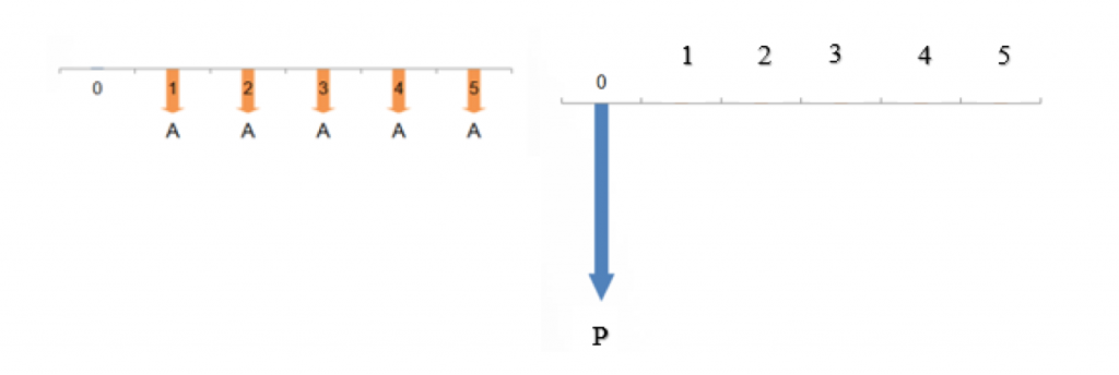
A uniform series, sometimes called an equal-payment series, is a cash flow series in which the same amount of money is paid or received in two or more sequential periods, as shown in Figure 3.4. These types of equal payments are also referred to as annuities.

This type of cash flow series is probably familiar to you: many long-term loans, such as house mortgages and car loans, involve a fixed monthly payment for a set length of time. These arrangements allow buyers to spread out payments on large purchases (like cars and houses) that would be difficult for most people to buy in one lump-sum.

An example of a uniform series is illustrated by a cash flow diagram below:

Uniform Cash Flow Series with Negative Cash Flows Diagram — Fig. 3.4 Uniform Cash Flow Series with Negative Cash Flows

We can analyze equal payment series scenarios in four different ways. These formulas can be used to convert uniform cash flows into an equivalent single cash flow, or distribute a single cash flow into an equivalent uniform series. For further information on how these formulas were developed, refer to Section 3.4.7 for the full derivation.

Present-value-from-payment formula: used to calculate the present value, P, from the regular payment A (given A, find P).

$P = A [\frac{(1+i)^N-1}{i(1+i)^N}]$ (3.9)

This formula can be used to answer questions such as “how much can I borrow to buy a car if I can afford monthly payments of $500?”

Payment-from-present-value formula: used to calculate the regular payment, A, from the present value P (given P, find A). This is used when distributing a large lump-sum value into smaller, equal payments.

$A = P [\frac{i(1+i)^N}{(1+i)^N-1}]$ (3.10)

For example, “how much will my monthly car payment be if I borrow $10 000 to buy a car now and plan to pay it back over 5 years?”

Future-value–from-payment formula: used to calculate the future value, F, from the regular payment A (given A, find F). It is commonly used to determine how much an account or loan will be worth after N periods of regular contributions.

$F + A[\frac{(1+i)^N-1}{i}]$ (3.11)

As an example: “if I save $500 every month, how much money will I have 5 years from now?”

Payment-from-future-value formula: used to calculate the regular payment, A, from the future value F (given F, find A). This formula is useful when trying to calculate the size of payment required to have a certain amount, F, in the future.

$A = F[\frac{i}{(1+i)^N-1}]$ (3.12)

For example, “if my goal is to have $10,000 in 5 years, how much will I have to put into my savings account each month?”

An important note regarding timeframes: in the above formulas, N denotes the number of periods in the uniform series, i denotes the interest (or discount rate) per period, and A denotes the equal cash flow per period. N, i, and A must all be in the same time frame. If an example requires calculating a monthly payment (A), then N must be months and i must be the monthly interest rate.

Note that calculating the present value of a uniform series will place the present value one period before payments begin. As shown in the cash flow diagram (Figure 3.4), if payments start in period 1, then P occurs in period 0.

Let’s look at some examples.

Uniform Series Example #1

Aladdin wants to borrow $12,000 and pay it off in equal monthly payments over a 5-year period. If the monthly interest rate is 0.75%, compounded monthly, how much would each payment be?

Solution

N = 5 years or 60 months,
i = 0.75% = 0.0075, and
P = $12,000.

To solve for A:

$A = P \left[\frac{i(1+i)^N}{(1+i)^N -1}\right] = \$ 12000 \left[\frac{0.0075(1+0.0075)^{60}}{(1+0.0075)^{60} - 1}\right] = \$ 249.10$

Thus, the monthly payment would be $249.10. Notice, this means Aladdin ends up actually paying a total of $14 946 for his $12 000 loan ($249.10*60), where $2 746 is the total interest paid to the lender on top of the loan.

Uniform Series Example #2

Brook wants to start saving for retirement. She plans to deposit $500 per month into a savings account that earns 6% per year (compounded annually). How much money will Brook have in the account after 25 years?

Solution

Here, we have monthly payments and we need to find the future value of the account, so we will use the future-value-from-payment formula 3.11.

But note the units: we are dealing with monthly payments, but interest is applied annually. This means we must use the end of period convention – treat all monthly deposits within each year as if they were all deposited on the last day of the year (discussed in Front material).

So, we have:

A = ($500/month)(12 months/year) = $6000/year
i = 6% per year
N = 25 years

$F = A \left[\frac{(1+i)^N - 1}{i}\right] = \$ 6000\left[\frac{(1+0.06)^{25} - 1)}{0.06}\right] = \$ 329 187.07$

So, after 25 years, Brook will have $329 187.07 in her account. Note that without any interest she would have only saved up $150 000 ($6000 per year x 25 years). Interest more than doubled the money!

Defered Annuity Example

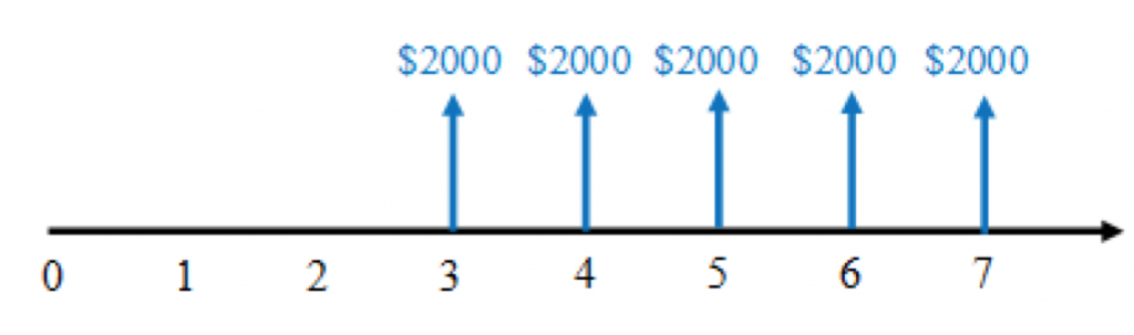
Given the schedule of cash flows in Figure 3.5, calculate the present value, at period 0, using an annual discount rate of 7%.

Deferred Annuity Cash Flow Series Diagram — Fig. 3.5 Deferred Annuity Cash Flow Series

Solution

In this case, we have A, and need to find P, so we will use the present-value-from-payment formula 3.9. But note: this formula will give us the present value in period 2 (see Figure 3.6). We need to then “move” it to period 0 (see Figure 3.7).

Step 1: Find the present value (P2) of the uniform series.

A = $2000
i = 7%
N = 5 years

$P_2 = A [\frac{(1+i)^N-1}{i(1+i)^N}] + \$ 2000 [\frac{(1.07)^5-1}{0.07(1.07)^5}] + \$ 8200.39$

Finding the P2 Cash Flow of the Uniform Series Diagram — Fig. 3.6 Finding the P2 Cash Flow of the Uniform Series

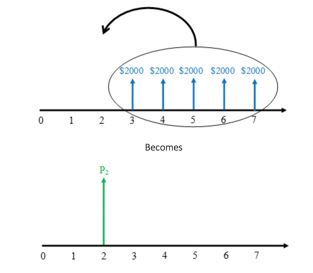
Step 2: Discount the P2 cash flow to period 0.

Now that we have a single cash flow at period 2, we can discount it to obtain the present value at period 0:

$P_0 = \frac{P_2}{(1+i)^N} = \frac{ \$ 8200.39}{(1.07)^2} = \$ 7162.54$

Discounting of the p2 Cash Flow Diagram — Fig. 3.7 Discounting of the p2 Cash Flow

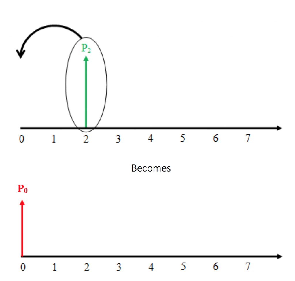
Therefore, the value of the uniform series at period 0 is $7162.54.

3.4.3 Linear Gradient Series

A linear gradient series is a series of cash flows which increase or decrease by a constant amount every period. An illustrative example is found in Figure 3.8 below.

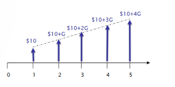
Linear Gradient Series Graph — Fig. 3.8 Linear Gradient Series

As we see, in each period the amount is increasing by $5. This is the gradient G. In the cash flow diagram above, the cash flow in period 1 is $10. In the second period, we add G to obtain a value of $15. In the third period, we add two times the gradient to get a cash flow of $20… and so on. Note that in Figure 3.8 cash flows are increasing due to a positive G. However, G can also be negative, so that each subsequent payment will be smaller than the previous one by G.

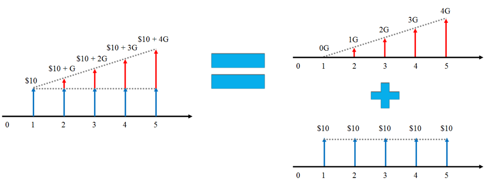
When calculating the linear gradient series, we must break up the cash flows into two series: a uniform series and a linear gradient series with a cash flow of zero in period 1, as shown below. In the Figure 3.8, A would be $10 and G would be $5.

Two-Step Analysis of the Linear Cash Flow Series Diagram — Fig. 3.9 Two-Step Analysis of the Linear Cash Flow Series

Notes on using the linear gradient series:

As with the uniform series that calculating the present value of a linear gradient series places the present value one period before the cash flows begin; if cash flows begin in period 1, the P will occur in period 0.
N is the number of interest periods, including the period in which the gradient’s cash flow is zero.
G can be positive or negative. If the cash flows are increasing each period, then G is positive; if they are decreasing, then G is negative.
A is always equal to the cash flow in the first period.

Formulas for analyzing a linear gradient series:

Present value of a linear gradient series: used to calculate the present value (in period 0) of a linear gradient portion of the series beginning in period 1 (given G, find P).

$P = G \left[\frac{(1+i)^N - iN - 1}{i^2 (1+i)^N}\right]$ (3.13)

This formula along with the corresponding uniform series formula can be used to answer questions such as: “what is the present value of a 10 year maintenance contract for which the payments increase by $1000 per year?”

Future value of a linear gradient series: used to calculate the value of a linear gradient portion of the series at the end of the last period in the series (given G, find F).

$F = G \left[\frac{(1+i)^N - iN - 1}{i^2}\right]$ (3.14)

This formula along with the corresponding uniform series formula can be used to determine, for example: “if I open an account and make deposits increasing the amount deposited by $100 each month, how much will I have in the account after 24 months?”

Converting a linear gradient series to a uniform series: used to convert a linear gradient series to a uniform series with the same payment timing (given G, find A).

$A = G \left[\frac{(1+i)^N - iN - 1}{[i(1+i)^N - 1]}\right]$ (3.15)

After adding this result to the uniform portion of the cash flow series, this formula can answer questions, such as: “how much would I have to pay if I were to make equal monthly payments on a loan instead of increasing each payment by $100 each month for the next 12 months?”

To see how these formulas were derived refer to Section 3.4.7.

Note that, as before, i is the discount or interest rate per period and N is the number of periods.

Do not forget that these formulas only apply to the gradient portion of the series. If the series in the problem is split into a gradient series and a uniform series as discussed in this section, then the value of the uniform series must be added to the gradient series value to get the total value of the series.

Let’s see some examples of how these formulas are applied.

Linear Gradient Series Example #1

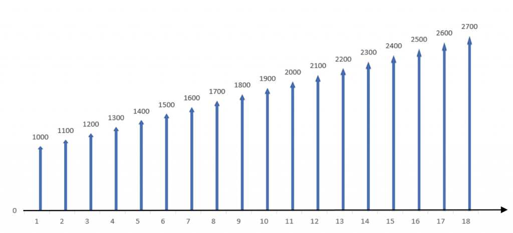
Gary decides to start saving for his newborn twin daughters’ post secondary education. He can afford to save $1000 in the first year, $1100 in the second year, $1200 in the third year, and so on, increasing the amount by $100 each year. The savings account pays 5% interest, compounded annually. How much money will he have in the account after 18 years?

Solution

Step 1: Draw the cash flows.

Step 2: Split up the cash flow series into two components.

Looking at the cash flow in this problem (Figure 3.10) we can see that it increases by a constant amount ($100) each, implying a linear gradient. The cash flow in the first period is not zero, so we must split the original cash flow schedule into a linear gradient series and a uniform series.

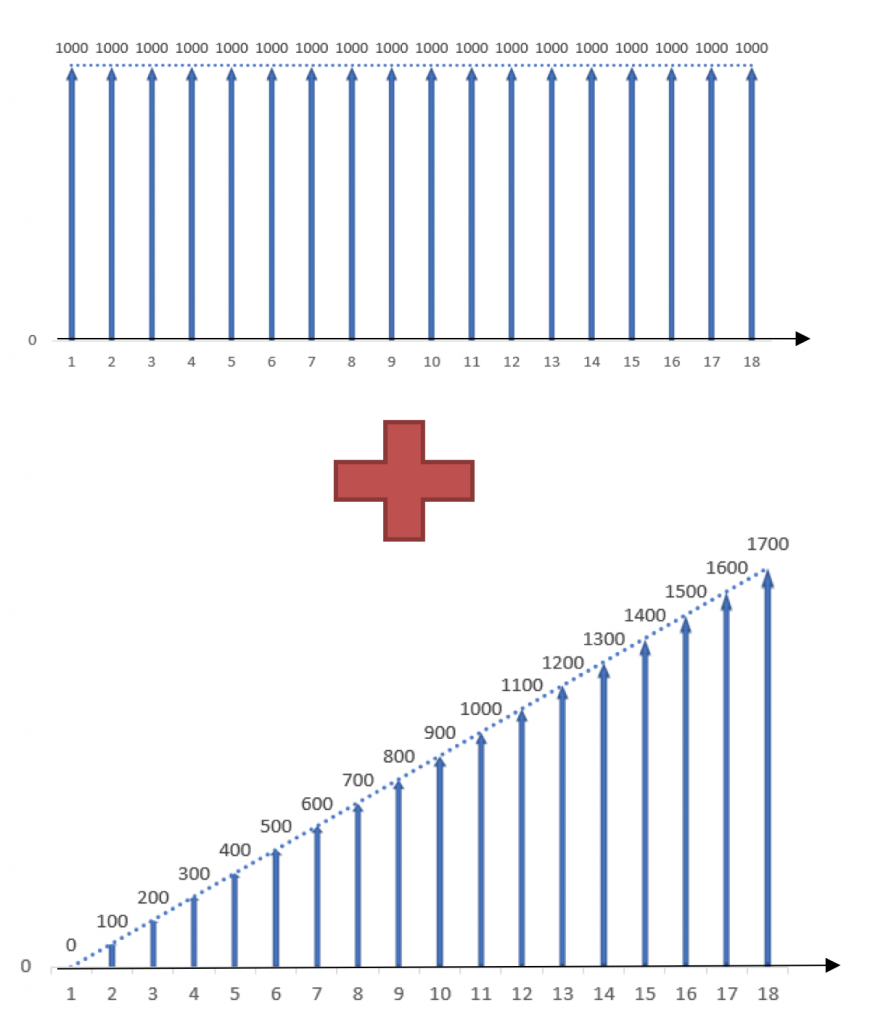
Uniform Series and Linear Gradient Series Diagram — Fig. 3.11 Uniform Series and Linear Gradient Series

The cash flows in the uniform series are equal to the savings in the first period – in this case, A = $1000. The gradient is positive, since the cash flows are steadily increasing. For the linear gradient series, G = $100.

Step 3: Verify that payments and interest rate have the same time units.

The account pays annual interest and deposits are made annually, so the values have the same time units.

A = $1000 per year
G = $100 per year
i = 5% per year
N = 18 years

Step 3: Calculate the future values of the linear gradient and uniform series using formulas 3.14 and 3.11.

$F_{grad} = G[\frac{(1+i)^N - iN - 1}{i^2}] = \$ 100 [\frac{(1+0.05)^18 - (0.05)(18)-1}{0.05^2}] = \$ 20,264.77$

$F_{uniform} = A[\frac{(1+i)^N - 1}{i} = \$ 1000 [\frac{(1+0.05)^18 - 1}{0.05}] = \$ 28,132.38$

Step 4: To calculate the total future value after 18 years, add the future values of the uniform series and the linear gradient series.

$F_{total} = F_{gradient} + F_{uniform} \\ F_{total} = \$ 20,264.77 + \$ 28,132.38 = \$ 48,397.15$

Thus, after contributing $33 300to the account for 18 years, Gary will have saved $48 397.15 for his daughters’ education.

Linear Gradient Series Example #2

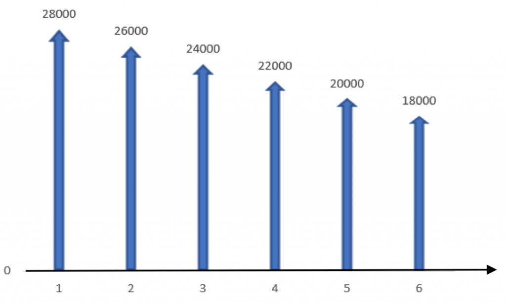
A machine shop is planning to buy a CNC (computer numerical controlled) mill to automate simple steps for large-scale production jobs, saving labour costs. The mill costs $100 000. Using the mill would result in the following labour cost savings:

Year	1	2	3	4	5	6
Savings ($)	28000	26000	24000	22000	20000	18000

If the company’s discount rate is 8%, should the mill be purchased?

Solution

Step 1: Draw cash flows. Note that these values are savings. In situations like this we assume that total cost, which is not stated, remains constant throughout. As a result, these savings also imply that profits increase by the same amount. So we can draw the cash flow diagram as follows:

Step 2: Separate the cash flows into a uniform series and a linear gradient series.

Looking at the cash flow in this problem (Figure 3.12), we can see that it decreases by a constant amount ($2000) each year throughout the life of the machine, implying a linear gradient. The cash flow in the first period is not zero, so we must split the original cash flow schedule into a linear gradient series and a uniform series.

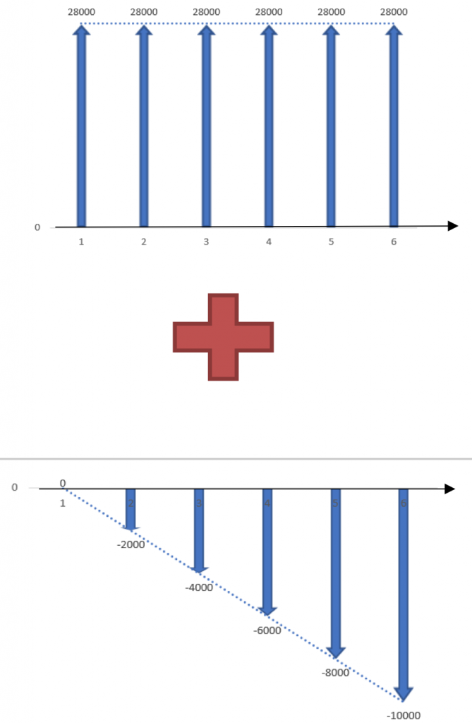
The cash flows in the uniform series are equal to the savings in the first period, so in this case, A = $28,000. The gradient is negative, since the cash flows are steadily decreasing. Thus, G = –$2000.

Step 3: Verify that payments and interest rate have the same time units.

Savings in this example are projected on the annual basis and we have an annual discount rate, so the values have the same time units.

A = $28,000 per year
G = -$2000 per year
i = 8% per year
N = 6 years

Step 4 : To determine if the mill is a good investment, we need to find the present value of the overall cash flow series by adding the present values of the two components. We use formulas 3.9 and 3.13 to find present values:

$P_{overall} = P_{gradient} + P_{uniform}$

$P_{overall} = G \left[\frac{(1+i)^N - iN - 1}{i^2(1+i)^N}\right] + A \left[\frac{(1+i)^N - 1}{i(1+i)^N}\right]$

$P_{overall} = -\$ 2000\left[\frac{(1+0.08)^6 - (0.08)(6) - 1}{0.08^2 (1+0.08)^6}\right] + \$ 28000 \left[\frac{(1+0.08)^6 - 1}{0.08(1 + 0.08)^6}\right]$

$P_{overall} = -\$ 21 046.55 + \$ 129 440.63 = \$ 108 394.08$

Therefore, since the present value of the savings, $108 394.08, is greater than the cost of the mill, $100 000, purchasing the mill is a good financial investment. Even though the difference of the present value of the savings and the cost of the mill is only $8394.08, the actual saving from the mill are $138 000.

3.4.4 Geometric Gradient Series

The geometric gradient series is a series of cash flows in which each cash flow increases (or decreases) by a constant percentage (in contrast to the linear gradient series, where each cash flow increases or decreases by a constant amount). The percentage change is called the geometric gradient, denoted by g. The cash flow values are calculated similarly to compound interest: if the cash flow in the first year is A1, then in the second year the cash flow will be A1(1 + g), in the third year it is A1(1 + g)2, and so on. This is illustrated in the cash flow diagram below.

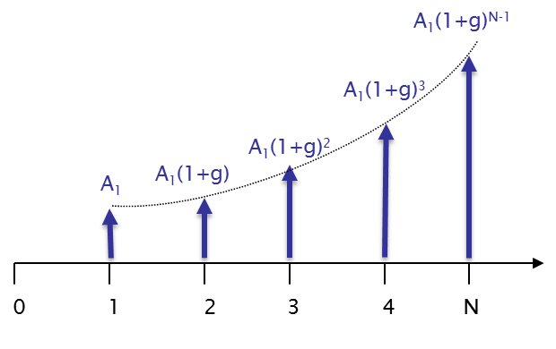
Geometric Gradient Series diagram — Fig. 3.14 Geometric Gradient Series

As evident from Figure 3.14, just like in the case with compound interest, geometric gradient results in exponential growth. Thus, cash flows are highly sensitive to the gradient value.

The gradient g can be positive or negative. Positive values of g lead to a rise in subsequent cash flows, while negative values of g cause the cash flows to decrease over time. To find P we need to “move” all of the cash flows to period 0.

The first step in solving the gradient portion of the series is to check whether the geometric gradient (g) is equal to the discount rate (i). If they are not equal, the formulas are:

When $i \neq g$ :

$P = \frac{A_1}{i-g}[1 - (\frac{1+g}{1+i})^N]$ (3.16)

$F = \frac{A_1}{i-g}[(1+i)^N-(1+g)^N]$ (3.17)

If they are equal, the denominator of the first term on the right-hand side of each equation will equal 0 and cannot be solved. Thus, the following formulas need to be used instead:

When $i = g$

$P = A_1(\frac{N}{1+i})$ (3.18)

$F= NA_1(1+i)^N-1$ (3.19)

These formulas are used to answer questions such as: “what is the present (or future) value of a project that is expected to yield $1000 in profit this month, and the profit is expected to increase by 5% every following month for 11 months?”

Important note: be careful not to confuse i and g. The geometric gradient, g, is the rate at which the cash flows increase or decrease in subsequent periods, which reflects changes in the nominal value of the cash flows. The discount rate, i, is used to account for the time value of money.

When using the geometric gradient series formulas:

N is the number of interest periods, including the initial period where the gradient is equal to zero.
The discount rate, i, and the gradient, g, must be specified. The MARR (which will be covered in chapter 5) is often used as the discount rate.
The cash flow is NOT divided into uniform and gradient components. It can be solved directly using the above formulas.

Let’s see some example problems where geometric gradient series formulas are used.

Geometric Gradient Series Example

Brad, a civil engineer, is coordinating a project to build a new stadium in Regina. The cost of stadium construction is estimated to be $278 million.[6]Part of the sum will be collected in the form of grants from the Provincial Government, the City of Regina and the Saskatchewan Roughriders. The rest, which amounts to $100 million, will be loaned by the Province for a period of 30 years at 3.5% interest, compounded annually. The loan is to be repaid on a monthly basis with equal payments throughout the entire term.

The City will use ticket sales revenues for some of the events held at the stadium to make the loan payments. In the first year, the revenues are expected to be equal to the total loan payments for the year. The project management team expects these revenues to increase by 5% each year.

Does the present value of the total revenue from ticket sales exceed the value of the loan? (Assume 6% discount rate)

Solution

First, we need to determine the monthly loan payments, so that we can determine how much is to be repaid in the first year, which also tells us the expected ticket revenues in the first year. Thus, we will solve this problem in two stages: calculating the equal payments of the loan and calculating the total revenues from ticket sales.

Part 1:

Step 1: To calculate the equal payment value, we use the payments-from-present value formula 3.10. We have the following information:

N = 30,
i = 3.5% = 0.035, and
$P_{loan}$ = $100 million.

To solve for A:

$A = P_{loan}[\frac{i(1+i)^N}{(1+i)^N-1}] + \$ 100 million [\frac{0.035 \ast (1+0.035)^{30}}{(1+0.035)^{30}-1}] = \$5.44 million$

So, the annual loan payments are $5.44 million.

Part 2:

Step 3: Now that we know the value of the yearly loan payment, we can conclude that ticket sales in the first year are expected to be $5.44 million. Since, project management team expects the revenues to increase by 5% each year, this implies a geometric gradient series with the first cash flow A=A1=$5.44 million.

To find the present value of the total revenue from ticket sales at the end of 30 years, the present value formula for geometric series is used. Note that , so we use formula 3.16 to calculate future value of the total revenue. Thus, we have:

N = 30,
i = 6% = 0.06
g = 5% = 0.05, and

A=A1=$5.44 million

$P_{total revenue}=\frac{A_1}{i-g}[1-(\frac{1+g}{1+i})^N]=\frac{\$5.44 million}{0.06-0.05}[1-(\frac{1+0.05}{1+0.06})^{30}]=\$544million[1-0.075] = \$ 136million$

So, the present value of the total revenue from ticket sales exceeds the value of the loan by $36 million.

3.4.5 Complex Cash Flows

The purpose of cash-flow equations is to simplify calculations required for cash flow analysis. It is usually much more convenient to group several cash flows together for one calculation rather than to discount each cash flow separately.

To apply the appropriate formulas, it is important to identify the type of cash flow series. However, in practice, it is not always apparent what type of series we are dealing with. Cash flows can be seemingly “random” or change drastically over the analysis period. We call these complex cash flows. To tackle complex cash flows problems, the trick is to seek out patterns in the cash flow schedules and “deconstruct” them into different cash flow series, which may allow us to use the cash-flow equations.

The example below demonstrates how complex cash flows can be approached.

A complex cash flow example

Given the schedule of cash flows in Figure 3.15, find the total present value of the series at year 0 using a discount rate of 8%.

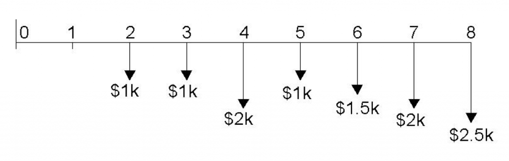
Schedule of Cash Flows Diagram — Fig. 3.15 Schedule of Cash Flows

To find the present value of this cash flow series, we must “move” each amount to year 0. One way to do so is to discount each cash flow one-by-one using the present-value formula 3.8 for single cash flows and sum them. However, it may be less time-consuming to recognize that the individual flows can be grouped into separate series.

Step 1: Examine the cash flow diagram for patterns. One set of patterns is as follows:

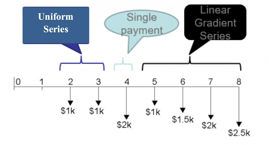
Grouping of the Cash Flows diagram — Fig. 3.16 Grouping of the Cash Flows

Note that this is not the only possible way to segment the cash flows, but this is the segmentation we will use to solve the problem.

Step 2: Now to calculate the total present value we will begin by moving each of the three series to period 0.

Segment A: The uniform series

The uniform series begins in year 2, so we calculate its “present” value from the uniform series formula 3.9 to get the series’ value in year 1, which we will call P1. Then, we move P1 to year zero by discounting it over one year (see Figure 3.17).

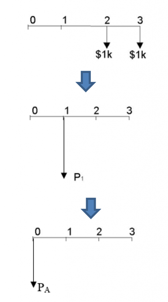
Discounting of a Uniform Series Diagram — Fig. 3.17 Discounting of a Uniform Series

$P_{1} = A\left[\frac{(1+i)^N - 1}{i(1+i)^N}\right] = -\$1000\left[\frac{(1+0.08)^2 - 1}{0.08(1+0.08)^2}\right] = -\$1783.26$

$P = \frac{P_{1}}{(1+i)} = \frac{-\$1783.26}{(1+0.08)} = -\$1651.17$

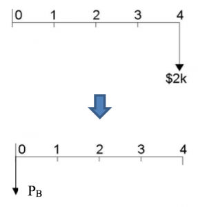
Segment B: The single payment

To determine the present value of the single payment in year 4 we discount it 4 years to bring it to the present, as shown in Figure 3.18:

Discounting of a Single Payment Diagram — Fig. 3.18 Discounting of a Single Payment

$P_B = \frac{F_{4}}{(1+i)^N} = \frac{=\$2000}{(1+0.08)^4} = -\$1470.06$

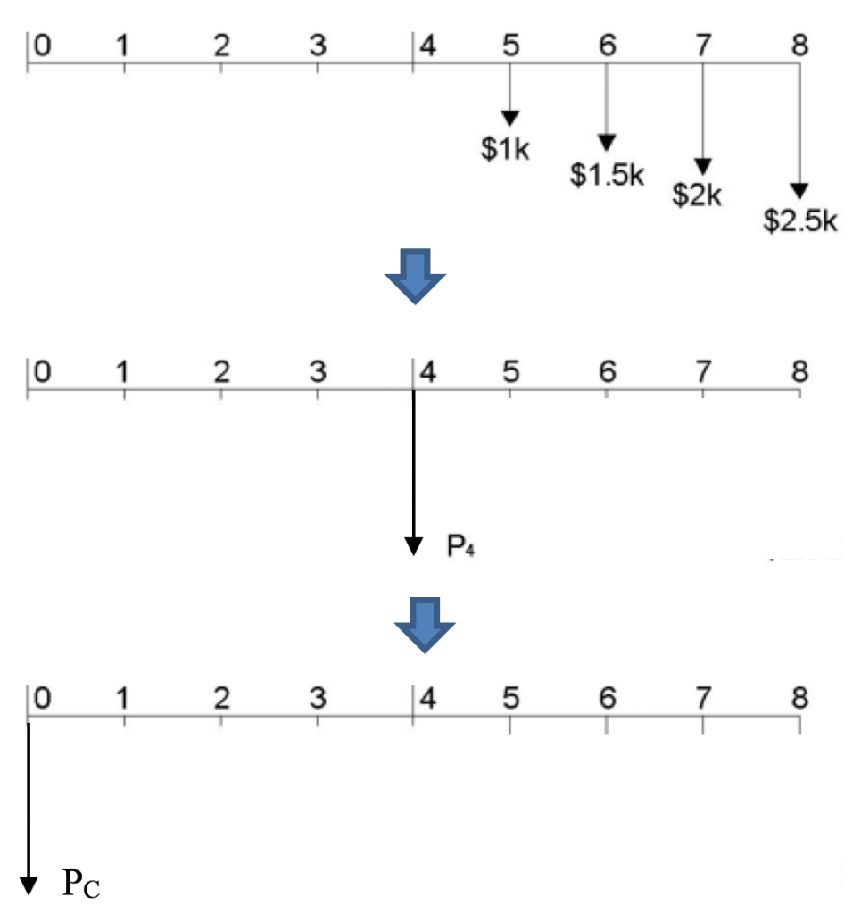
Segment C: The linear gradient series

Recall that linear gradient series must be split into two series: a uniform series and a gradient series. In this example, the first cash flow of the linear gradient series is -$1000, so the uniform series will have equal payments, A = -$1000. Each consecutive outflow increases by $500, so the gradient, G = -$500 (recall, we treat outflows as negative values). The first cash flow of the segment occurs at year 5, so when we use equations to calculate the present value, the resulting present value is actually in year 4. So we must remember to “move” it to year 0, as shown in Figure 3.19:

Discounting of a Linear Gradient Series Diagram — Fig. 3.19 Discounting of a Linear Gradient Series

$P_{4} = P_{uniform} + P_{gradient} = A\left[\frac{(1+i)^N - 1}{i(1+i)^N}\right]+G\left[\frac{(1+i)^N - iN - 1}{i^2(1+i)^N}\right]$

$= -\$1000\left[\frac{(1+0.08)^4 - 1}{0.08(1+0.08)^4}\right] - \$500\left[\frac{(1+0.08)^4 -(0.08)(4)-1}{0.08^2(1+0.08)^4}\right]$

$= -\$3312.13 - \$2325.05 = -\$5637.18$

We now “move” the year 4 present value to year 0:

$P_C = \frac{P_{4}}{(1+i)^N} = \frac{-\$5637.18}{(1+0.08)^4} = -\$4143.50$

Step 3: To obtain the present value of the complete series we sum the present values of each segment:

Total P = P_A+ P_B + P_C

Total P = (-$1651.17) + (-$1470.06) + (-$4143.50) = -$7264.73

So, the present value of the complete series (Total P) is -$7264.73.

3.4.6 Summary of Equations

The summary of equations of economic equivalence is in Table 3.4 below.

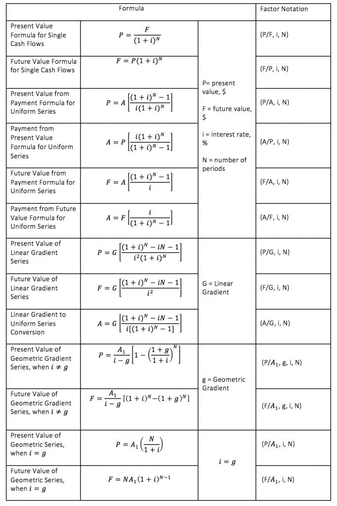
Equations of Economic Equivalence Formulas Table — Table 3.4 Equations of Economic Equivalence Formulas

The final column of this table shows what is called factor notation – a short-hand way of expressing the equations. For example, let’s take a look at the present value for the single cash flows formula (row 1).

$P = \frac{F}{(1+i)^N}$

So, $P/F=\frac{1}{(1+i)^N}$ . The right-hand side of this equation is called a factor. In factor notation this is shown as

$(P/F,i,N)$

This factor is read as “P divided by F, given i and N”.

So, to represent the entire equation, we write

$P = F (P/F, i, N)$

Similarly, using factor notation, the future this factor is expressed as (F/P, i, N), which is read as “F divided by P, given i and N”. The future value formula, thus, becomes:

$F = P(F/P, i, N)$

As you browse through the formulas in the table, you will notice that each equation requires multiplication involving a value of a cash flow (present value, future value, annuity, linear gradient) and a factor which depends on i and N (also g when dealing with geometric gradient series). To simplify calculations, factor values for different i and N have been tabulated in so-called compound interest factor tables for equations of economic equivalence. These tables allow to substitute already calculated factor values given interest-rate-and-number-of-periods scenarios in the appropriate formulas, hence decreasing the amount of necessary calculations.

3.4.7 Derivations

The following sections provides derivations for the formulas used in Section 3.4. These derivations are provided to help you understand how the equations were developed. The ability to independently arrive at these derivations is not essential to being able to use them correctly or have a solid understanding of economic equivalence.

Single cash flows formulas:

Future Value formula for single cash flows:

$F = P(1+i)^N$ (3.6)

1. Recall that the future value is equal to the present value and accumulated interest.	$F = P + I$
2. The interest earned in period 1, is equal to $I_1=Pi$ . So, the future value in period 1 becomes	$F_1 = P + I_1 = P + Pi = P(1 + i)$
3. In period 2, interest is applied to the ending balance in year 1, which is F₁: $I_2 = F_1i$ . Thus, the future value in period 2 is	$F_2 = F_1 + I_2 = F_1 + F_1i = F_1(1 + i)$
4. Since, from equation (2), F₁= $P(1 + i)$ , we can substitute this into equation (3), yielding	$F_2 = [P(1 + i)](1 + i)$
5. This simplifies to	$F_2 = P(1 + i)^2$
6. In period 3, interest is now applied to the present value in period 2, which is F2: $I_3 = F_2i$ . Hence, the future value in period 3 becomes	$F_3 = F_2 + I_3 = F_2 + F_2i = F_2(1 + i)$
7. Since, from equation (5) $F_2 = P(1 + i)^2$ , substituting the right-hand side from of the equation into equation (6) yields	$F_3 = P(1+i)^2(1 + i)$
8. Simplifying, we get	$F_3 = P(1 + i)^3$
9. Continuing for N periods using the same steps, we get the future value formula for single cash flows for N periods and interest rate i .	$F = P(1 + i)^N$

Present value formula for single cash flows (present value with compound interest formula):

$P =\frac{F}{(1 + i)^N}$ (3.8)

The present value formula can be obtained from the future value formula for single cash flows 3.6:

1. Recall the future value formula 3.6	$F = P(1 + i)^N$
2. To obtain P, we divide both sides by $(1 + i)^N$ . We now have the present value formula for single cash flows.	$P = \frac{F}{(1+i)^N}$

Uniform Series formulas:

Present-value-from-payment formula:

$P = A [\frac{(1+i)^N-1}{i(1+i)^N}]$ (3.9)

1. The present value is the sum of all discounted cash flows in the series. In a uniform series, each cash flow has a value of A.	$P = \frac{A}{1 + i}+\frac{A}{(1 + i)^2}\cdots+\frac{A}{(1 + i)^{N-1}}+\frac{A}{(1 + i)^N}$
2. Now we multiply both sides of the equation by $(1 +i)$ . On the right-hand side, all denominators’ exponents decrease by 1.	$(1 + i)P = A +\frac{A}{1 + i}\cdots+\frac{A}{(1 + i)^{N-2}}+\frac{A}{(1 + i)^N-1}$
3. We need to get the right-hand side in equation (2) from equation (1). To do that, first, we move $\frac {A}{(1+i)^N}$ to the left-hand side in equation (1).	$P - \frac{A}{(1 + i)^N}=\frac{A}{1+i}+\frac{A}{(1+i)^2}\cdots+\frac{A}{(1+i)^{N-1}}$
4. We then add A to both sides of equation (3), which yields equation (4).	$P+A-\frac{A}{(1+i)^N}=A+\frac{A}{1+i}+\frac{A}{(1+i)^2}\cdots+\frac{A}{(1+i)^{N-1}}$
5. Now, we relate equations (1) and (4) to obtain an equation without series (5).	From (1) and 3) $(1+i)P = P + A - \frac{A}{(1+i)^N}$
6. We now rearrange the terms in equation (5) to solve for $P$ .	$(1+i)P = P + A - \frac{A}{(1+i)^N} \rightarrow iP = A [1 - \frac{1}{(1+i)^N}] \rightarrow P= \frac {A}{i}[1 - \frac{1}{(1+i)^N}]$
7. Multiplying the terms inside the brackets in equation (6) by i we obtain the present-value-from-payment formula (7).	$P = A [\frac{(1+i)^N-1}{i(1+i)^N}]$

This formula combined with the present-value formula for single cash flows 3.8 is used to derive the three remaining formulas: the payment-from-present value formula 3.10, the future-value-from-payments formula 3.11 and the payment from future value formula 3.12.

Payment-from-present-value formula:

$A = P [\frac{i(1+i)^N}{(1+i)^N-1}]$ (3.10)

The payment-from-present-value formula 3.10 and the present-value-from-payment formula 3.9 are reciprocals of each other:

1. Recall the present-value-from-payment formula 3.9	$P = A [\frac{(1+i)^N-1}{i(1+i)^N}]$
2.To obtain A, we divide both sides by $[\frac{(1+i)^N-1}{i(1+i)^N}]$	$A = P\frac{1}{[\frac{(1+i)^N-1}{i(1+i)^N}]}$
3. Rearranging equation (2) we get the payment-from-present-value formula	$A = P[\frac{i(1+i)^N}{(1+i)^N-1}]$

Future-value–from-payment formula:

$F = A[\frac{(1+i)^N-1}{i}]$ (3.11)

This formula can be obtained using the payment-from-present value formula 3.9 and the future value for single cash flows formula 3.6:

1. Recall the present-value-from-payment formula 3.9	$P = A [\frac{(1+i)^N-1}{i(1+i)^N}]$
2. Next, recall the present value formula for single cash flows 3.8	$P =\frac{F}{(1 + i)^N}$
3. Substituting $\frac{F}{(1+i)^N}$ from equation (2) in equation (3) yields	$\frac{F}{(1 + i)^N}=A [\frac{(1+i)^N-1}{i(1+i)^N}]$
4. Now we multiply both sides of equation (3) by $(1+i)^N$	$F = A[\frac{(1+i)^N-1}{i(1+i)^N}](1+i)^N$
5. This, in turn, cancels out $(1+i)^N$ in the denominator in the term in square brackets on the right-hand side in equation (4). We get the future-value-from-payment formula	$F = A[\frac{(1+i)^N-1}{i}]$

Payment-from-future-value formula:

$A = F[\frac{i}{(1+i)^N-1}]$ (3.12)

The payment-from-future-value formula 3.12 and the future-value-from-payment formula 3.11 are reciprocals of each other:

1. Recall the future-value-from-payment formula 3.11	$F = A[\frac{(1+i)^N-1}{i}]$
2. Solving for A, we divide both sides by $[\frac{(1+i)^N-1}{i}]$	$A = F\frac{1}{[(1+i)^N-1}{i}]$
3. Rearranging equation (2) we get the payment-from-future-value formula	$A = F[\frac{i}{(1+i)^N-1}]$

Linear Gradient Series Formulas:

These formulas apply to the gradient series with linear gradient G as illustrated in Figure 3.20.

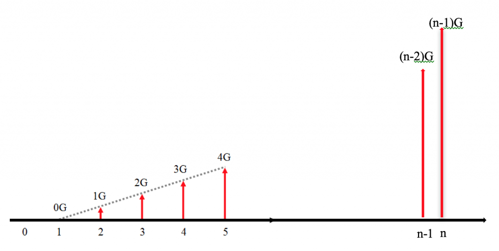
Linear Gradient Series Diagram — Fig. 3.20 Linear Gradient Series

Future value of a linear gradient series formula:

$F = G[\frac{(1+i)^N-i_N-1}{i^2}]$ (3.14)

1. Future value of the linear gradient series can be thought of as a sum of future values of individual cash flows in the series: 0G, 1G, 2G…(n-2)G, (n-1)G. Let i be the discount rate for discounting cash flows. The future value of the gradient series can thus be expressed as	$F = G(1+i)^{N-2}+2G(1+i)^{N-3}+\cdots +(n-2)G(1+i)^1+(n - 1)G$
2. Now we multiply both sides of the equation (1) by $(1+i)$ and factor out G. We will need this equation after the next step.	$F(1+i) = G[(1+i)^{N-1}+2(1+i){N-2}+ \cdots + (n-1)(1+i)]$
3. We go back to equation (1) again and now we only factor out G	$F=G[(1+i)^{N-2}+ \cdots +(n-2)(1+i)+(n-1)]$
4.Next, we subtract equation (3) from equation (2). 4.1 We rearrange the terms on the right-hand side of the equation by writing the terms that include $(1+i)$ with the same power from equation (2) and (3) next to each other. This allows us to subtract and rearrange them next. 4.2 We leave the first term in the brackets; subtract the next two, obtaining $(2-1)(1+i)^{n-2}$ as a result; we factor out $(1+i)$ from the two terms after the ellipsis getting $(1+i)(n-1-n+2)$ ; and leave the last term in the equation. 4.3 Further opening the brackets and simplifying the equation we get equation (4)	$F(1+i) - F = G[(1=i)^{N-1} + 2(1+i)^{N-2} = \cdots + (n-1)(1+i)] - G[(1+i)^{N-2}+ \cdots +(n-2)(1+i)^i+(n-1)]$ $\rightarrow F+iF-F=G[(1+i)^{n-1}+2(1+i)^{N-2}-91+i)^{N-2}+\cdots +(n-1)(1+i) - (n-2)(1+i) - (n-1)]$ $\rightarrow iF = G[(1+i)^{N-1} + (2-1)(1+i)^{N-2}+\cdots+(1+i)(n-1-n+2)-(n-1)]$ $\rightarrow iF = G[(1+i)^{N-1} + (1+i)^{N-2}+\cdots +(1+i)-n+1]$
5. Now we carry n out of the brackets in the right-hand side of equation (5)	$\rightarrow iF = G[(1+i)^{N-1}+(1+i(^{N-2}+\cdots+(1+i)+1]-nG$
6. Notice that the expression in the square brackets is geometric series, where the first term of the series is $(1+i)^{N-1}$ and each subsequent term is multiplied by $\frac{1}{(1+i)}$ . We can find the sum of the geometric series using the geometric series formula $\sum_{K=0}^{n-1}(ar^k)= a(\frac{1-r^n}{1-r})$ , where $a=(1+i)^{N-1}$ and $r=\frac{1}{(1+i)}$ . We write down the geometric series summation formula and substitute the values from the series in equation (5). After some algebraic manipulation, we obtain the sum of the geometric series, which is expressed by equation (6).	$\sum_{K=0}^{n-1}(ar^k) = (1+i)^{N-1}[\frac{1-(\frac{1}{1+i})^N}{1-\frac{1}{1+i}}]$ $\rightarrow\sum_{K=0}^{n-1}(ar^k) = (1+i)^{N-1}[\frac{1-(\frac{1}{1+i})^N}{\frac{1+i-1}{1+i}}]$ $\rightarrow\sum_{K=0}^{n-1}(ar^k) = (1+i)^{N-1}[\frac{1-(\frac{1}{1+i})^N}{\frac{i}{1+1}}]$ $\rightarrow\sum_{K=0}^{n-1}(ar^k) = (1+i)^{N-1}[\frac{1-(\frac{1}{1+i})^N}{i}(1+i)]$ $\rightarrow\sum_{K=0}^{n-1}(ar^k) = [\frac{1-(\frac{1}{1+i}^N}{i}\frac{(1+i)^{N-1}}{(1+i)}]$ $\rightarrow\sum_{K=0}^{n-1}(ar^k) = [\frac{1-(\frac{1}{1+i}^N}{i}(1+i)^N]$ $\rightarrow\sum_{K=0}^{n-1}(ar^k) =[\frac{(1+i)^N - \frac{(1+i)^N}{(1+i)^N}}{i}]$ $\rightarrow\sum_{K=0}^{n-1}(ar^k) =[\frac{(1+i)^N -1}{i}]$
7. Now we substitute equation (6) in equation (5) to get rid of the series in the equation	$iF = G[\frac{(1+i)^N-1}{i}]-NG$
8. Next, we solve for F by dividing both sides of equation (7) by i and rearranging the terms on the right-hand side of the equation, obtaining the future value of a linear gradient series formula	$F = \frac{G}{i}[\frac{(1+i)^N-1}{i}]-NG$ $\rightarrow F = \frac{G}{i}[\frac{(1+i)^N-1}{i}-N]$ $\rightarrow F = G[\frac{(1+i)^N - iN - 1}{i^2}]$

Present value of a linear gradient series formula:

$P = G [\frac{(1+i)^N-iN-1}{i^2(1+i)^N}]$ (3.13)

The present value of a linear gradient series formula 3.13 can be obtained from the present value formula for single cash flows 3.8 and future value of a linear gradient series formula 3.14:

1. Recall the future value of a linear gradient series formula 3.14	$F = G[\frac{(1+i)^N-i_N-1}{i^2}]$
2. To obtain P, we divide both sides by from the present value formula for single cash flows 3.8 $P = \frac{F}{(1+i)^N}$	$P = G [\frac{(1+i)^N-iN-1}{i^2}]\frac{1}{(1+i)^N}$
3. Multiplying the two fractions, we get the present value of a linear gradient series formula	$P = G [\frac{(1+i)^N-iN-1}{i^2(1+i)^N}]$

Converting a linear gradient series to a uniform series formula:

$A = G [\frac{(1+i)^N-iN-1}{i[(1+i)^N-1]}]$ (3.15)

This formula can be derived from the present value of the linear gradient series formula 3.13 and the present-value-from-payment formula 3.9:

1. Recall the present value of a linear gradient series formula 3.13	$P = G [\frac{(1+i)^N-iN-1}{i^2(1+i)^N}]$
2. Also recall the present-value-from-payment formula 3.9	$P = A [\frac{(1+i)^N-1}{i(1+i)^N}]$
3. We now substitute the right-hand side from equation (2) into the left-hand side of equation (1)	$A [\frac{(1+i)^N-1}{i(1+i)^N}] = G [\frac{(1+i)^N-iN-1}{i^2(1+i)^N}]$
4. To solve for A, we divide both sides of equation (3) by $\frac{(1+i)^N-1}{i(1+i)^N}$	$A = G[\frac{(1+i)^N-iN-1}{i^2(1+i)^N}][\frac{1}[{\frac{(1+i)^N-1}{i(1+i)^N}]}]$
5. Rearranging and simplifying equation (4) we get the formula for converting linear gradient series to a uniform series	$A = G [\frac{(1+i)^N-iN-1}{i^2(1+i)^N}][\frac{i(1+i)^N}{(1+i)^N-1}]$ $\rightarrow A = G[\frac{(1+i)^N - iN-1}{i[(1+i)^N-1]}]$

Geometric Gradient Series Formulas:

When $i \neq g$

Present value for geometric gradient series formula:

$P = \frac{A_1}{i-g}[1-(\frac{1+g}{1+i})^N]$ (3.16)

1.The present value of the geometric gradient series can be expressed as a sum of discounted values of individual cash flows in the series A1, A1(1+g), A1(1+g)² … A1(1+g)^N-1. Let i be the discount rate for discounting cash flows. The present value of the gradient series can thus be expressed as	$P = \frac{A_1}{(1+i)^1}+\frac{A_1(1+g)^1}{1=i)^2}+\frac{A_1(1+g)^2}{(1+i)^3} +\cdots+\frac{A_1(1=g)^{N-1}}{(1+i)^N}$
2. We now factor out A₁ in equation (1). We will need this equation after the next step.	$P = A_1[\frac{1}{(1+i)^1}+\frac{(1=g)^1}{(1+i)^2}+\frac{(1+g)^2}{(1+i)^3}+\cdots+\frac{(1+g)^{N-1}}{(1+i)^N}]$
3. Now we multiply both sides of the equation (2) by $\frac{1+g}{1+i}$ .	$P\frac{(1+g)}{(1+i)} = A_1[\frac{(1+g)}{(1+i)^2} + \frac{(1+g)^2}{(1+i)^3}+\frac{(1+g)^3}{(1+i)^4} +\dots+\frac{(1=g)^N}{(1+i)^{N+1}}]$
4. Next, we subtract equation (2) from equation (3). On the right-hand side of the equation, we rearrange the terms in brackets, placing same terms from equations (2) and (3) next to one another. Notice, that other than the first and the last terms in brackets, all the other terms will cancel out. So, rearranging the equation and canceling out the terms we get equation (4)	$P\frac{(1+g)}{(1+i)}-P=A_1[\frac{(1+g)}{(1+i)^2} + \frac{(1+g)^2}{(1+i)^3}+\frac{(1+g)^3}{(1+i)^4} +\dots+\frac{(1=g)^N}{(1+i)^{N+1}}]$ $-A_1[\frac{(1+g)}{(1+i)^2} + \frac{(1+g)^2}{(1+i)^3}+\frac{(1+g)^3}{(1+i)^4} +\dots+\frac{(1=g)^N}{(1+i)^{N+1}}]$ $\rightarrow P[\frac{(1+g)}{(1+i)} - 1] = A_1[-\frac{1}{1+i}+\frac{(1+g)}{(1+i)^2}+ \frac{(1+g)^2}{(1+i)^3}-\frac{(1+g)^2}{(1+i)^3}+ \frac{(1+g)^3}{(1+i)^4}+\cdots - \frac{(1+g)^{N-1}}{(1+i)^N} + \frac{(1+g)^N}{(1+i)^{N+1}}]$ $\rightarrow P[\frac{1+g)}{(1+1)} - 1] = A_1[\frac{(1+g)^N}{(1=i)^{N+1}} - \frac{1}{1+i}]$
5. Now we solve for P. First, we divide both sides of the equation by $[\frac{1+g}{1+i} - 1]$ = $\frac{1+g-1-i}{1+i} = \frac{g-i}{1+i}$	$P [\frac{g-i}{1+i}] = A_1 [\frac{(1+g)^2}{(1+i)^{N+1}} - \frac{1}{1+i}]$ $\rightarrow P = A_1[\frac{(1+g)^N}{(1+i)^{N+1}} - \frac{1}{1+i}][\frac{1+i}{g-i}]$
6. Canceling out (1+i) in equation (5) and further rearranging and simplifying the equation, we get the present value for geometric gradient series formula for the case when $i \neq g$ .	$P = A_1[\frac{(1+g)^N}{(1+i)^{N+1}} - \frac{1}{1+i}][\frac{1+i}{g-i}]$ $\rightarrow P = A_1[\frac{(1+g)^N}{(1+i)^N} - 1][\frac{1}{g-i}]$ $\rightarrow P = A_1[\frac{A_1}{g-i}[(\frac{1+g}{1+i})^N -1]$ $\rightarrow P+\frac{A_1}{i-g}[1-(\frac{1+g}{1+i})^N]$

Future value for geometric gradient series formula:

$F = \frac{A_1}{i-g}[(1+i)^N - (1+g)^N]$ (3.17)

This formula can be derived from the present value for geometric gradient series formula 3.16 and the future-value-from-payment formula 3.6:

1. Recall the present value for geometric gradient series formula 3.16	$P = \frac{A_1}{i-g}[1-(\frac{1+g}{1+i})^N]$
2. To obtain F, we multiply both sides by $(1+i)^N$ from the future value formula for single cash flows 3.6 $F = (1+i)^NP$	$F = \frac{A_1}{i-g}[1-(\frac{1+g}{1+i})^N](1+i)^N$
3. Multiplying the terms in equation (2) and simplifying the equation, we get the future value for geometric gradient series formula for the case when $i \neq g$ .	$F = \frac{A_1}{i-g}[(1+i)^N - (1+g)^N]$

When $i = g$

When discounting the cash flows in the case where the discount (interest) rate is equal to the geometric gradient, $i = g$ , all the cash flows have the same present value. This is because the cash flows are increasing at the same rate as they are being discounted, thus maintaining the purchasing power of the cash flow. Therefore, the formulas for this case will be different, although the approach used to derive these formulas is the same.

Present value for geometric gradient series formula:

$P = A_1(\frac{N}{1+i}$ (3.18)

1. Like in the case where $i = g$ , the present value of the geometric gradient series can be expressed as a sum of discounted values of individual cash flows in the series. Now that the gradient and the discount rates are equal ( $i = g$ ), these cash flows are A1, A1(1+i), A1(1+i)2 … A1(1+i)N-1.The present value of the gradient series can thus be expressed as	$P = \frac{A_1}{i-g}[1-(\frac{1+g}{1+i})^N]$
2. To obtain F, we multiply both sides by $(1+i)^N$ from the future value formula for single cash flows 3.6 $F = (1+i)^NP$	$F = \frac{A_1}{i-g}[1-(\frac{1+g}{1+i})^N](1+i)^N$
3. Multiplying the terms in equation (2) and simplifying the equation, we get the future value for geometric gradient series formula for the case when $i \neq g$ .	$F = \frac{A_1}{i-g}[(1+i)^N - (1+g)^N]$

When $i = g$

When discounting the cash flows in the case where the discount (interest) rate is equal to the geometric gradient, , all the cash flows have the same present value. This is because the cash flows are increasing at the same rate as they are being discounted, thus maintaining the purchasing power of the cash flow. Therefore, the formulas for this case will be different, although the approach used to derive these formulas is the same.

Present value for geometric gradient series formula:

$P = A_1(\frac{N}{1+i})$ (3.18)

1. Like in the case where $i \neq g$ , the present value of the geometric gradient series can be expressed as a sum of discounted values of individual cash flows in the series. Now that the gradient and the discount rates are equal ( $i = g$ ), these cash flows are A1, A1(1+i), A1(1+i)2 … A1(1+i)N-1.The present value of the gradient series can thus be expressed as

$P = \frac{A_1}{(1+i)^1}+\frac{A_1(1+i)^1}{(1+i)^2}+\frac{A_1(1+i)^2}{(1+i)^3}+\cdots+\frac{A_1(1+i)^{N-1}}{(1+i)^N}$

$\rightarrow P = \frac{A_1}{(1+i)^1}+\frac{A_1}{(1+i)^1}+\frac{A_1}{(1+i)^1}+\cdots+\frac{A_1}{(1+i)^1}$

2. We now factor out A1 in equation (1).

$P = A_1[\frac{1}{(1+i)^1}+\frac{1}{(1+i)^1}+\frac{1}{(1+i)^1}+\cdots+\frac{1}{(1+i)^1}]$

3. On the right-hand side of equation (2) we have N terms, each being $\frac{1}{(1+i)^1}$ . The sum of these terms is $\frac{N}{(1+i)^1}$ . Substituting this expression into equation (2) yields the

$P = A_1[\frac{N}{1+i}]$

Future value for geometric gradient series formula:

$F = NA_1(1+i)^{N-1}$ (3.19)

This formula can be derived from the present value for geometric gradient series formula 3.18 and the future-value-from-payment formula 3.6:

1. Recall the present value for geometric gradient series formula 3.18

$P = A_1(\frac{N}{1+i})$

2. To obtain F, we multiply both sides by $(1+1)^N$ from the future value formula for single cash flows 3.6 $F = P(1+i)^N$

$F = A_1(\frac{N}{1+i})(1+i)^N$

3. Multiplying the terms in equation (2) and simplifying the equation, we get the future value for geometric gradient series formula for the case when $i = g$ .

$F = A_1N[\frac{(1+i)^N}{1+i}]$

$\rightarrow F= NA_1(1+i)^{N-1}$

[6] Note amounts in this problem are indicated in US dollars, so the amount in Canadian dollars will differ. However, this is irrelevant to the problem

License

Icon for the Creative Commons Attribution 4.0 International License