
5.3 Analysis Period and Project Lives
Earlier in this chapter, we used NPV and AEV analysis to evaluate and compare several projects. However, the projects we considered were reasonably straightforward – the project durations were specified, and projects being compared had equal durations. That is, if a company needed equipment for 5 years, we would compare alternatives with 5-year project durations. But what happens when this is not the case?
For example, suppose that a custom 3D-printing company needs to choose the model of 3D printers it will use to fill customer orders. The company wants to plan for the next 10 years, but the two printers they are considering have useful lives of 4 years and 6 years. Even if we know the purchase prices and maintenance costs of the two printer models, how could we evaluate them appropriately? This section will discuss how we can adapt evaluation methods like AEV and NPV to these situations.
But first, here are two key definitions:
- Analysis period (also called the planning horizon or study period) is the length of time over which the project will occur, and over which we must analyze the project’s cash flows to make an economic evaluation. In the 3D-printing example the analysis period is 10 years because that is the length of time over which the company wishes to plan its finances.
- Project life (or project duration) is how long the project will last. In the 3D-printing example there are two projects to choose from: one with a project life of 4 years, and another with a project life of 6 years. After the project life has ended, the equipment is no longer useful to the company and must be either replaced or sold. The dollar amount the equipment can be sold for is the salvage value.
If alternatives have:
- unequal project lives, or
- project lives that are different than the analysis period
These differences need to be accounted for in our analysis. That is, we cannot simply evaluate the alternatives using NPV, AEV, or IRR analysis. We must adjust our methods depending on the situation. To properly analyze these problems, we must first be able to recognize the type of situation we are facing.
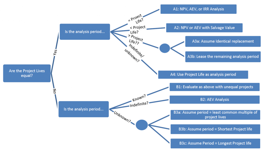
There are two important questions to consider for any case we analyze.
- Do our alternatives have equivalent project lives?
- Are the project lives equal to our chosen analysis period?
Figure 5.6 below shows the cases we might face depending on our answers to those two questions, and the suggested method of evaluation for each case. These cases and their solutions will each be discussed in greater detail.
Equivalent Project Lives
5.3.1 A1: Project Lives = Analysis Period
The simplest analysis problems are those in which all project lives are equal to each other and equal to the analysis period. You are already familiar with this type of problem, as the majority of Chapter 5 has exclusively dealt with this scenario. These problems can be solved directly with NPV, AEV, or IRR analysis, and require no special treatment of the cash flows. For more examples of these problems, please refer to the NPV, AEV, or IRR analysis sections.
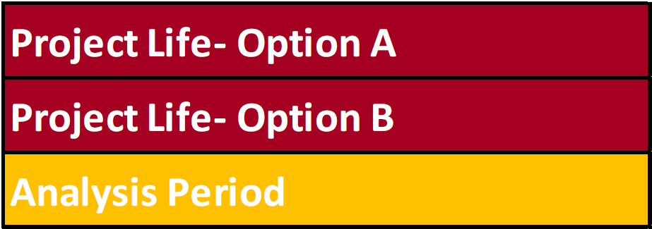
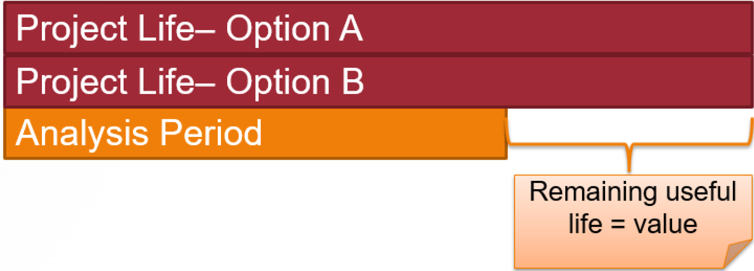
5.3.2 A2: Equal Project Lives > Analysis Period
When all alternatives have equal project lives but last longer than the analysis period, the projects will still have some value remaining at the end of the analysis period. This is the salvage value discussed in the Capital Recovery Cost (CRC) Method. For example: you are trying to choose between two cars which last longer than you need them to, so you sell them at the end of your analysis period and incorporate that salvage value in your analysis. A salvage value is treated as a positive single cash flow occurring at the end of the analysis period, and included in the NPV or AEV analysis like any other cash flow.
Two types of situations may occur: you may be given the salvage value, or it may not be known. First, let’s consider an example where the salvage values are given to us.
Case 1: Given Salvage Value
In some circumstances, such as with an automobile or a commonplace piece of equipment, it may be possible to estimate a future salvage value with reasonable accuracy. In these situations, we can apply the given salvage value as a single cash flow at the end of the project during our calculations. Consider the following example:
Example 1: Given Salvage Value
Mark has rented additional farmland on a 5-year lease, and needs to purchase a new combine harvester to expand his operations. He can either purchase a new combine for $480,000 or a used combine for $160,000. The increased profits from the additional combine are unknown, but Mark knows they will be identical regardless of which combine he purchases. He expects the new combine to have maintenance costs of $2500 per year and sell for $250,000 after 5 years. He also estimates that the used combine will have annual maintenance costs of $8000 and sell for $85,000 after 5 years. If Mark uses a MARR of 12% for his farm, should he buy new or used?
Find the NPV of each combine, including purchase price, maintenance costs, and salvage value. Incorporate the linear series cash flow formula in order to calculate the maintenance costs.
![NPV_{NEW} = P_{NEW} + A_{NEW}\left[\frac{(1+i)^N-1}{i(1+i)^N}\right] + \frac{F_{NEW}}{(1+i)^N}](https://openpress.usask.ca/app/uploads/quicklatex/quicklatex.com-aafb39e192c4182f82ea02a966f4444a_l3.png "Rendered by QuickLaTeX.com")
![NPV_{NEW} = -\$480,000 - \$2500 \left[\frac{(1+0.12)^5-1}{0.12(1+0.12)^5}\right] + \frac{\$250,000}{(1+0.12)^5}](https://openpress.usask.ca/app/uploads/quicklatex/quicklatex.com-8097af1878a2e2e35bdb5e50a4ffb6f9_l3.png "Rendered by QuickLaTeX.com")

![NPV_{USED} = P_{USED} + A_{USED}\left[\frac{(1+i)^N-1}{i(1+i)^N}\right] + \frac{F_{USED}}{(1+i)^N}](https://openpress.usask.ca/app/uploads/quicklatex/quicklatex.com-7361e0bd1ade57eb4e4b8fbeca2ea7df_l3.png "Rendered by QuickLaTeX.com")
![NPV_{USED} = -\$160,000 - \$8000 \left[\frac{(1+0.12)^5-1}{0.12(1+0.12)^5}\right] + \frac{\$85,000}{(1+0.12)^5}](https://openpress.usask.ca/app/uploads/quicklatex/quicklatex.com-989ca7eb549efa9c34b5e2f867aa3a84_l3.png "Rendered by QuickLaTeX.com")

Since the used combine has a higher NPV, Mark should purchase the used machine for his farm. Note that since Mark’s revenues from this new purchase are unknown, it is unclear whether even this lowest cost alternative will be profitable for him.
Salvage Value Unknown
Sometimes, salvage values are unknown and must be estimated. We assume that the investment (e.g. a piece of equipment) decreases in value by roughly the same amount each year. This allows us to use as the linear depreciation method, which is based on linear interpolation, to estimate its salvage value at any point in time.
The formula to find salvage value (S) for a project using this method is shown below, where C is the initial investment cost. (Note that this equation can also be generalized to find the salvage value at any point during the project life)

While linear depreciation is a common method, it does not apply in all cases. Historical data may show that the depreciation rate is non-linear. One of the most common examples of this case is cars: the value of a new car will decrease dramatically during the first year of ownership, and more gradually in the longer term. We will not do any examples of this kind here, but a similar concept is covered in Chapter 2.4 relating to depreciation.
Let’s see an example using the linear depreciation method.
Example 2: Salvage Value Unknown
A candy manufacturing plant is looking to replace its toffee-pulling machine. Two different companies (Mr. Fantastic & Co. and Stretch Armstrong Inc.) sell basic toffee-pulling machines with the same essential features. The chosen machine will be operated for the next 7 years.
| Machine | Initial Cost | Annual Maintenance Costs |
| Mr. Fantastic | $10,000 | $1,000 |
| Stretch Armstrong | $13,000 | $600 |
Each machine has a useful life of 8 years. If the company’s MARR is 9%, which machine should be chosen?
Solution
In this problem, both models have a project life (useful life) of 8 years, which is longer than the analysis period (7 years). So, we must use salvage values at the end of the analysis period to compare the two models. However, no salvage values are given in the problem statement, so we will estimate their salvage values based on the assumption that their value decreases linearly over time.
To find the salvage values at the end of year 7, we use the equation above.


Now that we have the salvage values of the two models, we can compare their NPVs. Remember to include the salvage value as a positive cash flow at year 7.

![NPV = P + A \left[ \frac{(1+i)^N-1}{i(1+i)^N} \right] + \frac{F}{(1+i)^N}](https://openpress.usask.ca/app/uploads/quicklatex/quicklatex.com-b511261c539f33133f2e9afd50cdc80c_l3.png "Rendered by QuickLaTeX.com")
![NPV_{Fantastic} = -\$10,000 -\$1000 \left[ \frac{(1+0.09)^7-1}{0.09(1+0.09)^7} \right] + \frac{\$1250}{(1+0.09)^7} = -\$14,349.16](https://openpress.usask.ca/app/uploads/quicklatex/quicklatex.com-c191c95b41ccf3410d05177bd0299ed1_l3.png "Rendered by QuickLaTeX.com")
![NPV_{Stretch} = -\$13,000 -\$600 \left[ \frac{(1+0.09)^7-1}{0.09(1+0.09)^7} \right] + \frac{\$1625}{(1+0.09)^7} = -\$15,130.84](https://openpress.usask.ca/app/uploads/quicklatex/quicklatex.com-01e700cce1985644f0c1ee396656ae22_l3.png "Rendered by QuickLaTeX.com")
Because the Mr. Fantastic machine has a higher net present value (that is, it will ultimately cost less than Stretch Armstrong), Mr. Fantastic should be chosen.
5.3.3 A3: Equal Project Lives < Analysis Period
In some cases, we need to consider several project alternatives whose project lives are equal and shorter than the analysis period. In these cases, the alternatives do not last long enough, so something must be done to cover the remaining portion of the analysis period.
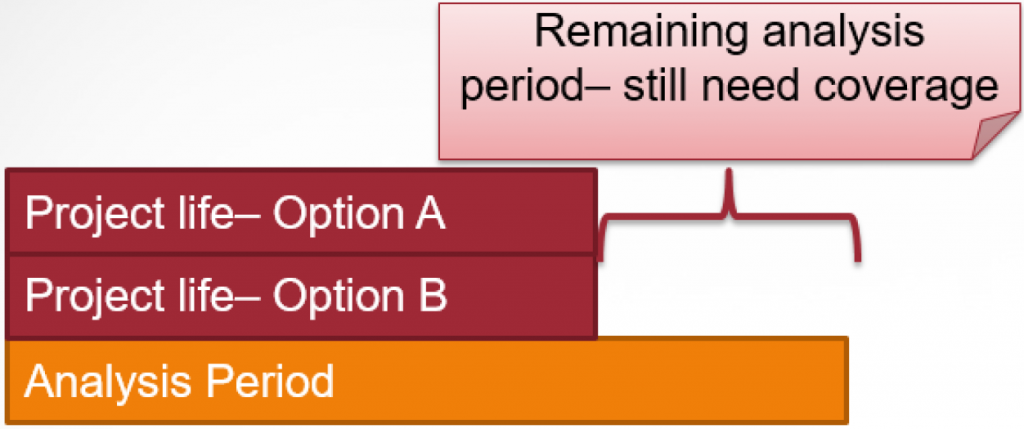
The remaining time in the analysis period can be solved by two methods. You can cover the remaining analysis period by assuming:
- Each item is replaced with repeated, identical items until the end of the analysis period; or
- Leasing is used to cover the remainder of the analysis period.
The method chosen to compare an alternative should be applied to all others for consistency. If you use the replacement method for Option A then the replacement method must also be used for Option B.
A3a: Repeated Projects
This method assumes that it is possible to repeat the chosen project with identical cash flows until the end of the analysis period, such as in the illustration below:
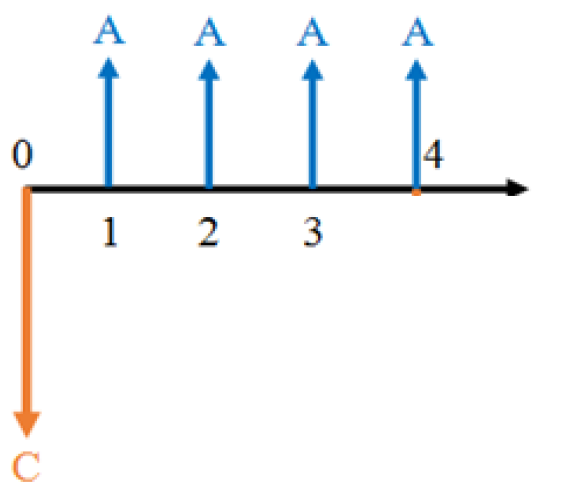
The cash flows for Project A, with a four-year project life:
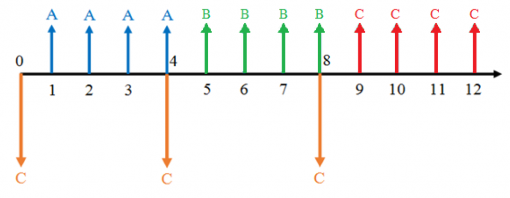
The cash flows for Projects A, B, and C: identical four-year projects repeated over 12 years.
This illustration shows three repetitions of a project that consists of an initial cost followed by equal revenues in the following four years. Each time the project is repeated, the initial cost of the new project must be paid in the last year of the previous project. Consider a taxi driver who replaces their vehicle every three years. They will need to buy a new vehicle at the end of each three year cycle, so they can earn money from that vehicle for each of the following three years.
When repeating projects this way, we can calculate the NPV of the entire set of repeated projects needed to cover the analysis period. We can also use the NPV to obtain an AEV if desired. (Note that the AEV of a set of repeated projects should be the same as the AEV of just one copy of the project.)
Another issue arises, however, in situations where the analysis period is not a multiple of the project life (e.g. the project life is 4 years and the analysis period is 10 years). When the project life does not divide evenly into the analysis period, the last repetition of the project will be cut short – so we use a salvage value! Below is an illustration of the same cash flows as the previous example, but with the salvage value at year 10:
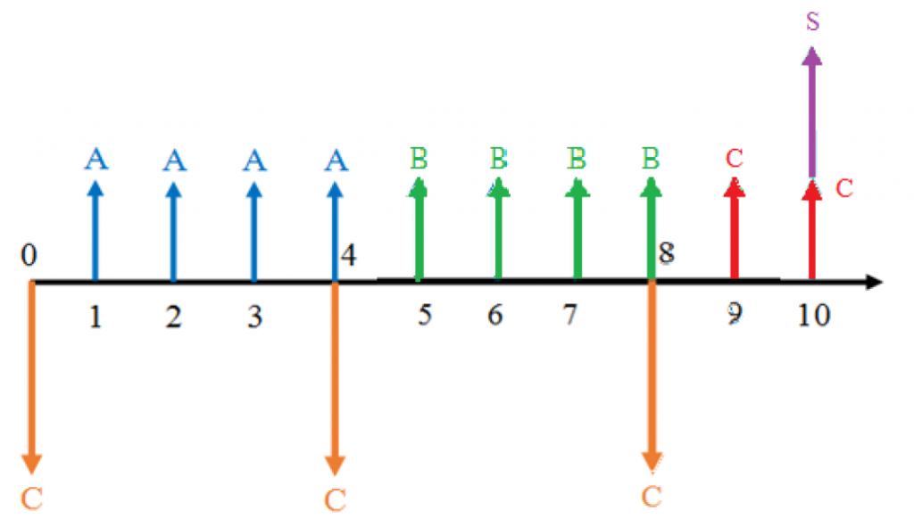
As we can see from the above diagram, an analysis period of 10 years would require 3 copies of a 4-year project. The third copy would be salvaged for its remaining value at the end of the analysis period.
If the salvage value is not given, we can estimate it using the linear formula from the previous section.
Example
Alyson runs an international shipping company that is adding a new trade route, which requires adding another container ship to their fleet. She must choose between two ships, as shown in the table below: Boaty McBoatFace, which is faster and more expensive, or Shippy McShipFace, which is slower and less expensive.
| Model | Initial Cost | Annual Earnings |
| Boaty McBoatFace | $30 million | $2 million |
| Shippy McShipFace | $20 million | $1 million |
Each model has a useful life of 10 years, after which the salvage cost is cancelled out by the decommissioning cost (i.e. there is zero salvage value). However, she needs to operate this route for the next 24 years. If the company’s MARR is 4%, which ship should Alyson choose?
Solution
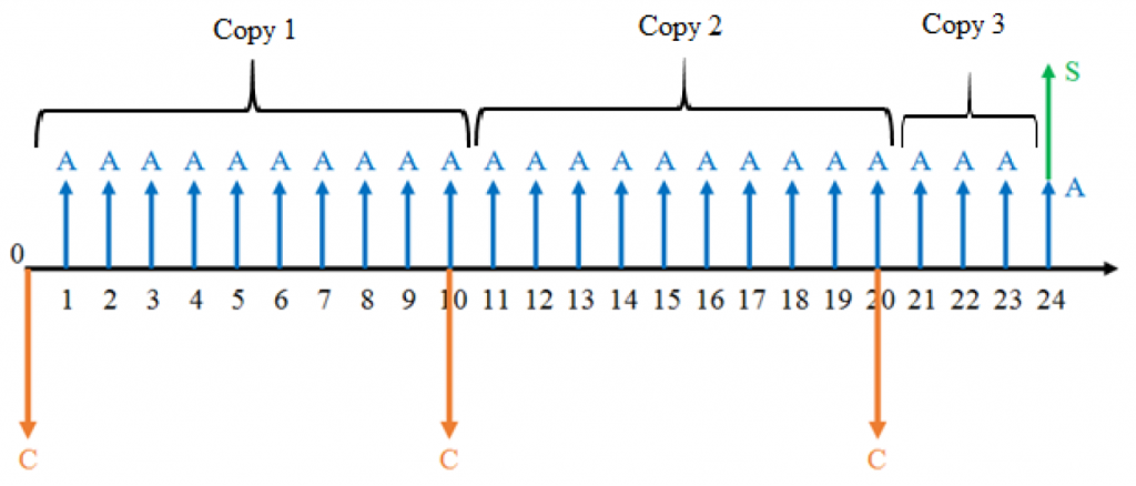
Although both models have useful lives of 10 years, the analysis period for this problem is 24 years. This means that whichever model Alyson chooses, she must use a total of 3 copies of the project (the ship), and salvage the last one at the end of the 24th year – or 4 years into its life. The cash flows for either model would look like this:
1 – Calculate the salvage values that she can expect in the 24th year.


2 – Now that we have the salvage values of the two models, we can compare their NPVs.

![NPV = -\$\text{30 million}\left( 1+\frac{1}{1.04^{10}}+\frac{1}{1.04^{20}}\right) + \$\text{2 million}\left[\frac{1.04^{24}-1}{0.04(1.04^{24})}\right] + \frac{\$\text{18 million}}{1.04^{24}}](https://openpress.usask.ca/app/uploads/quicklatex/quicklatex.com-2e8db19fb931ff49868735475e829bf6_l3.png "Rendered by QuickLaTeX.com")

![NPV = -\$\text{20 million}\left( 1+\frac{1}{1.04^{10}}+\frac{1}{1.04^{20}}\right) + \$\text{1 million}\left[\frac{1.04^{24}-1}{0.04(1.04^{24})}\right] + \frac{\$\text{12 million}}{1.04^{24}}](https://openpress.usask.ca/app/uploads/quicklatex/quicklatex.com-577d8f469904999ff1365139f765e09f_l3.png "Rendered by QuickLaTeX.com")

Because Shippy McShipFace ultimately has a lower cost, Shippy McShipFace should be chosen.
A3b: Leasing
When using repeated projects to fill an analysis period, relying on the salvage value of the final project is not always the most economical option. Another way we can ensure coverage for the entire analysis period is by leasing the needed equipment. We still repeat the chosen project as needed, but we only repeat the project whenever we can use its entire useful life. Once the remainder of the analysis period is shorter than the useful life of the chosen alternative, we cover the remainder with leasing.
Consider a project with a 4 year duration being applied over a 10 year analysis period. Using leasing, the cash flows for the scenario would look like this:
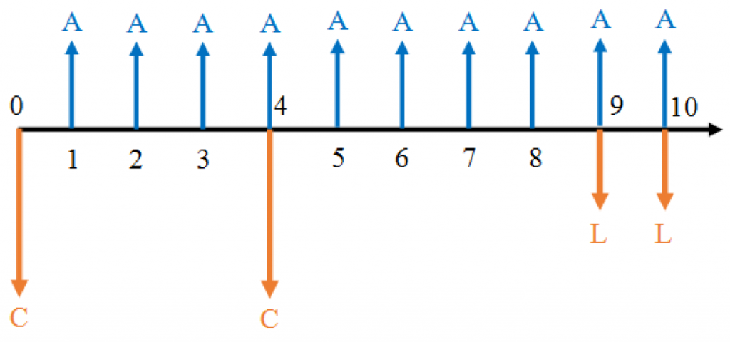
In the above diagram, the cash flows labelled 𝐿𝐿 represent lease payments for the equipment. As we can see, the project life is 4 years, which does not divide evenly into the 10-year analysis period. Under the leasing method, we use the same project twice, beginning in year 0 and year 4. This covers the first 8 years. Purchasing another project, however, would require salvaging the project after the 10th year. Instead, we use leasing to cover the 9th and 10th years.
5.3.4 A4: Equal Project Lives with Indefinite Analysis Period
For some cases, like a highway or other major infrastructure project, the analysis period for the project may be practically indefinite, or at least unknown. In such cases, we have no defined cut-off point at which to salvage projects or begin a lease. Since we need a baseline for comparing alternatives, the project life is used as the analysis period. We can then apply a basic evaluation method such as NPV or AEV, which will reduce the problem to a form that we are now familiar with.
Unequal Project Lives
Analysis becomes quite different when at least one alternative has a different useful life than the others. When this is the case, special steps must be taken to ensure the cash flows are evaluated properly.
When project alternatives have unequal lives, there are three analysis cases to consider:
- the analysis period is known and considered finite, or
- the analysis period is considered indefinite, or
- the analysis period is unknown and considered finite
5.3.5 B1: Unequal Project Lives with Known Analysis Period
If the analysis period for a project is known, but project lives are unequal, the situation is not significantly different than with equal project lives; however, we must consider the projects separately. This is best shown by considering a simple example:
Your donut shop is considering three mutually exclusive donut-making-machines over an analysis period of 20 years. Machine A costs $20,000 and will earn $1600/year over a project life of 25 years. If it is salvaged 5 years early, its salvage value will be $2000. Machine B costs $5000 and will earn $1500/year over a project life of 4 years. It can also be repeated as many times as necessary. Machine C costs $17,000 and will earn $1475/year over a project life of 20 years. Assume a MARR of 5%. Which project should you invest in?
Since all three projects have different project lives, we must consider them all separately. We can use the same approaches for each independent project as we did for our equal project lives examples, and afterwards compare the NPV of each project.
For Machine A, the project life is longer than the analysis period, so we can conduct an NPV analysis with an added salvage value (as in A1).

![NPV_A = P_A + A_A \left[\frac{(1+i)^N-1}{i(1+i)^N}\right] + \frac{S_A}{(1+i)^N}](https://openpress.usask.ca/app/uploads/quicklatex/quicklatex.com-71c9f65a42bae26d66548530b9406777_l3.png "Rendered by QuickLaTeX.com")
![NPV_A = -\$20,000 + \$1600 \left[\frac{(1+0.05)^{20}-1}{0.05(1+0.05)^{20}}\right] + \frac{\$2000}{(1+0.05)^{20}}](https://openpress.usask.ca/app/uploads/quicklatex/quicklatex.com-ef77f7faa26ba8280d52845443cb5fbf_l3.png "Rendered by QuickLaTeX.com")

For Machine B, the project life is shorter than the analysis period, so we consider identical replacement projects for the entire analysis period (as in A2). So first, lets find the NPV of the machine over its 4 year project life:
![NPV_B = -\$5,000 + \$1500 \left[\frac{(1+0.05)^{4}-1}{0.05(1+0.05)^{4}}\right]](https://openpress.usask.ca/app/uploads/quicklatex/quicklatex.com-da78a0f3ab8bc102741728e165cc70a6_l3.png "Rendered by QuickLaTeX.com")

To fill the analysis period, we will require 5 identical machines, each contributing $318.93 every four years (note that the N values substituted in are therefore multiples of 4); we can find the total NPV of this option by considering all 5 machines:

For Machine C, the project life is equal to the analysis period (as in A3), so we calculate the NPV result as usual:
![NPV_C = \$17,000 + \$1475 \left[\frac{(1+0.05)^{20}-1}{0.05(1+0.05)^{20}}\right]](https://openpress.usask.ca/app/uploads/quicklatex/quicklatex.com-a246948c777345a9ed2847c1972f2b4b_l3.png "Rendered by QuickLaTeX.com")

We can see by comparing the NPVs of each project, that Machine C is the most lucrative and should be invested in.
5.3.6 B2: Unequal Project Lives with an Indefinite Analysis Period
Sometimes, we do not know exactly how long a project will be used, but we expect that it will be used for a very long time, perhaps indefinitely. This situation often arises with public infrastructure projects such as roads, parks, water distribution networks, Egyptian pyramids, etc. In these scenarios, the cash flows may be known, but we cannot select a reasonable analysis period. To solve these problems, we simply use AEV analysis.
Example
Your plastics manufacturing company wants to replace one of its injection moulds. You have two options:
- Mould A that lasts 5 years with an initial price of $5000, with maintenance costs of $500/yr
- Mould B that lasts 7 years with an initial price of $7000, with maintenance costs of $400/yr
If your company’s MARR is 6%, which option is cheaper? Assume that your company plans to be in business long term.
Solution
Because the problem statement tells us that the company plans to be in business long term, we assume the chosen mould will be used “indefinitely,”. Since the project lives are unequal, we will use AEV analysis. Let’s calculate the AEV of each alternative, and compare.
Remember that AEV gives an annual amount. If we look at the two mould options, we see that the maintenance costs are already in annual payments! This means that, instead of calculating the NPV of the maintenance costs and then converting to an AEV, we can just add the maintenance costs “as-is” to the AEV of the upfront cost.
Mould A
Maintenance costs: AA = -$500
Purchase price: PA = -$5000
i = 6%
N = 5 years
![AEV_A = P_A \left[\frac{i(1+i)^N}{(1+i)^N-1}\right] + A_A = -\$5000 \left[\frac{0.06(1+0.06)^5}{(1+0.06)^5-1}\right] - \$500 = -\$1686.98](https://openpress.usask.ca/app/uploads/quicklatex/quicklatex.com-b34f162250d26636b135e580d6e233ea_l3.png "Rendered by QuickLaTeX.com")
Mould B
Maintenance costs: AB = -$400
Purchase price: PB = -$7000
i = 6%
N = 7 years
![AEV_B = P_B \left[\frac{i(1+i)^N}{(1+i)^N-1}\right] + A_B = $7000 \left[\frac{0.06(1+0.06)^7}{(1+0.06)^7-1}\right] - \$400 = -\$1653.95](https://openpress.usask.ca/app/uploads/quicklatex/quicklatex.com-90e1f6f08b643353762017e89cc90afc_l3.png "Rendered by QuickLaTeX.com")
We can see that Mould B has a higher AEV (lower annual cost, in this case). Therefore, your company should choose Mould B.
5.3.7 B3: Unequal Project Lives with Finite Analysis Period
When the analysis period is considered finite, but is unknown, we must choose what it will be. There three options:
A) Analysis period = least common multiple (LCM) of project lives
B) Analysis period = shortest project life among alternatives
C) Analysis period = longest project life among alternatives
Often, this choice is entirely arbitrary and is based on the preference of the analyst. Note that the choice of analysis period should not affect the outcome of the analysis. In some fringe cases this might pose an issue; for example, suppose a winery purchased a very expensive, specialized piece of equipment for sealing casks of wine. Since the equipment is so specialized, there might be no second-hand buyers available, making the salvage value essentially zero. In this case, the equipment might be a valuable solution over 25 years, but extremely inefficient over 5 years compared to another option (e.g. paying labourers to seal the casks by hand) since its up front cost is so high. These sorts of scenarios are rare, however, and most often the same project will be preferable regardless of the chosen analysis period.
Let’s solve an example using each of the three methods listed above and compare the results.
Unequal Project Lives Example
Suppose that a city is replacing its fleet of garbage collection trucks. It is currently choosing between 3 models: the Truckasaurus, the Trashgobbler, and the Garbotron 3000. The city will replace all their trucks with trucks of the chosen model. The table below lists the costs associated with replacing the city’s fleet.
| Model | Initial Cost | Annual Maintenance Costs | Project Life |
| Truckasaurus | $5 million | $375,000 | 5 years |
| Trashgobbler | $4 million | $475,000 | 4 years |
| Garbotron 3000 | $10 million | $325,000 | 10 years |
If the city has a MARR of 5% per year, which model should be chosen?
Solution
Start by listing all given values. We will use C for initial costs and A for annual maintenance costs.
Truckasaurus: CA = $5 million, AA = $375,000/yr, Project life = 5 years
Trashgobbler: CB = $4 million, AB = $475,000/yr, Project life = 4 years
Garbatron: CC = $10 million, AC = $325,000/yr, Project life = 10 years
i = 5% per year for all options
The discount rate and the maintenance costs have the same time units, so we can proceed. However, all project lives are unequal, and the analysis period is unknown. Since we have to choose an analysis period, for this example we will perform the analysis three times, using each of the above methods once.
B3a: Analysis Period = Least Common Multiple of Project Lives
For the LCM method, we set the analysis period equal to the least common multiple of all project lives (in this case, it’s 20 years) and compare NPVs.
Step 1: Draw the cash flows for each project over the 20-year analysis period (values shown in millions).
Truckasaurus: 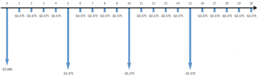
Trashgobbler: 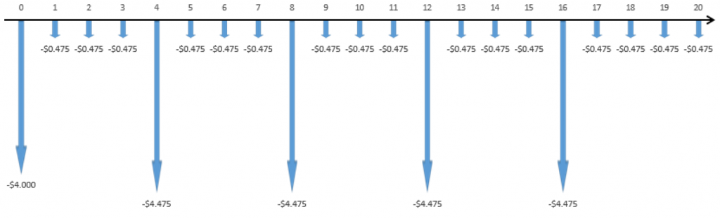
Garbotron 3000: 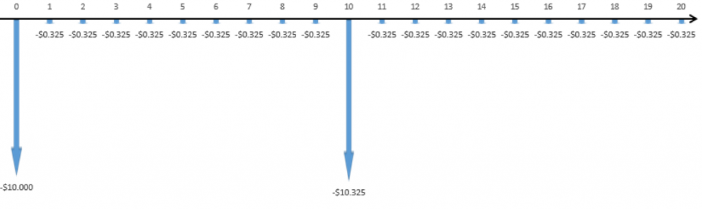
Step 2: Calculate the NPV of each alternative (watch those N values!).
![NPV_{Truck}= -\$ \text{5 million}\left( 1+\frac{1}{1.05^{5}}+\frac{1}{1.05^{10}}+\frac{1}{1.05^{15}}\right) -\$375,000 \left[ \frac{1.05^{20}-1}{0.05(1.05)^{20}} \right]](https://openpress.usask.ca/app/uploads/quicklatex/quicklatex.com-398d25c33bdbff5620d1fc4b8f0cfd73_l3.png "Rendered by QuickLaTeX.com")

![NPV_{Trash}= -\$ \text{4 million}\left( 1+\frac{1}{1.05^{4}}+\frac{1}{1.05^{8}}+\frac{1}{1.05^{12}}+\frac{1}{1.05^{16}}\right) -\$475,000 \left[ \frac{1.05^{20}-1}{0.05(1.05)^{20}} \right]](https://openpress.usask.ca/app/uploads/quicklatex/quicklatex.com-1c5a0b898e0d96065d3c6fbb4c6aba04_l3.png "Rendered by QuickLaTeX.com")

![NPV_{Garbo}= -\$ \text{10 million}\left( 1+\frac{1}{1.05^{10}}\right) -\$325,000 \left[ \frac{1.05^{20}-1}{0.05(1.05)^{20}} \right]](https://openpress.usask.ca/app/uploads/quicklatex/quicklatex.com-f6133e2a4fcf7287c912f48da67dd22e_l3.png "Rendered by QuickLaTeX.com")

From this method, we can see that the Truckasaurus is the best option.
B3b: Analysis Period = Shortest Project Life
For this method, we set the analysis period equal to the shortest project life among all the project alternatives (4 years, in this example). Note that the longer projects will still have some remaining useful life after 4 years. Therefore, we will need to use salvage values at the end of the analysis period. As these were not given, we will estimate these values in Step 2.
Step 1: Draw cash flows.
Truckasaurus: 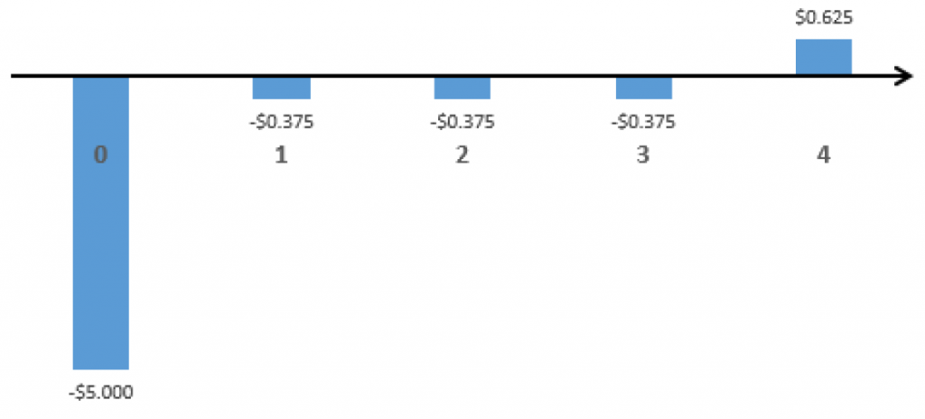
Trashgobbler: 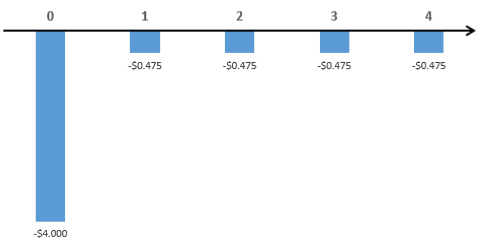
Garbotron 3000: 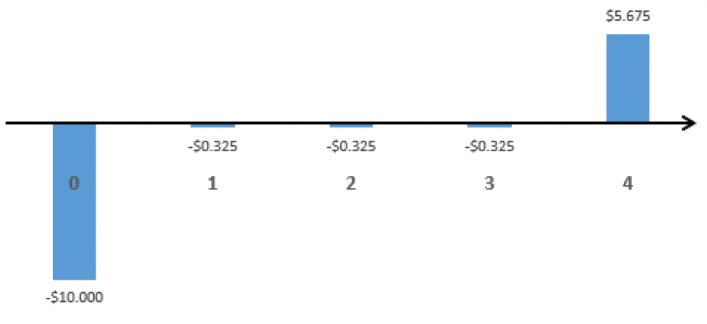
Step 2: Calculate salvage values for the Truckasaurus and Garbotron 3000.
Salvage values are not given in the problem statement, so we will estimate the salvage values using linear interpolation.


Step 3: Calculate all NPVs to compare projects using the following general equation:

So we have:
![NPV_{Truck} = -\$\text{5 million} - \$375,000 \left[ \frac{1.05^4-1}{0.05(1.05)^4} \right] + \frac{\$\text{1 million}}{1.05^4} = -\$\text{5.51 million}](https://openpress.usask.ca/app/uploads/quicklatex/quicklatex.com-134a9dceea5888a81b7b805ecd1ec66b_l3.png "Rendered by QuickLaTeX.com")
![NPV_{Trash} = -\$\text{4 million} - \$475,000 \left[ \frac{1.05^4-1}{0.05(1.05)^4} \right] = -\$\text{5.68 million}](https://openpress.usask.ca/app/uploads/quicklatex/quicklatex.com-171a1f9f80bc1bb86592a1d7d612061b_l3.png "Rendered by QuickLaTeX.com")
![NPV_{Garbo} = -\$\text{10 million} - \$325,000 \left[ \frac{1.05^4-1}{0.05(1.05)^4} \right] + \frac{\$\text{6 million}}{1.05^4} = -\$\text{6.22 million}](https://openpress.usask.ca/app/uploads/quicklatex/quicklatex.com-397cedf6a618e47fa177fb7c16033e8c_l3.png "Rendered by QuickLaTeX.com")
Again, we find that the Truckasaurus is the cheapest option.
B3c: Analysis Period = Longest Project Life
For this method, the analysis period will be equal to the longest project life among the alternatives, which is 10 years in this example. The Truckasaurus and Trashgobbler will be replaced by identical copies of themselves for the length of the analysis period. However, the Trashgobbler has a life of 4 years, which does not divide nicely into the 10-year analysis period. This means it will have to be repeated twice, and the third copy will have to be salvaged after the 10th year (its second year of use).
Step 1: Draw the cash flows.
Truckasaurus: 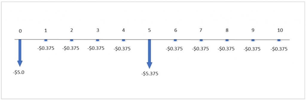
Trashgobbler: 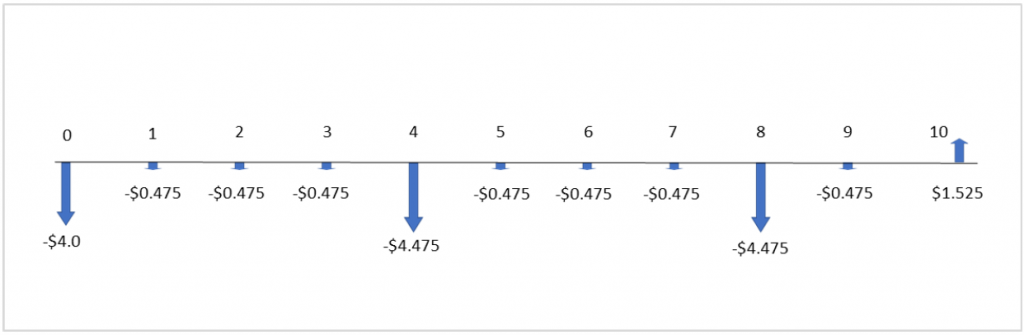
Garbotron 3000: 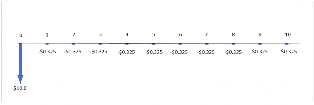
Step 2: Calculate the salvage value of the Trashgobbler.

Step 3: Calculate NPVs and compare.
![NPV_{Truck} = -\$\text{5 million}\left(1+\frac{1}{(1.05)^5} \right) - \$375,000 \left[ \frac{1.05^{10}-1}{0.05(1.05)^{10}} \right] = -\$\text{11.8 million}](https://openpress.usask.ca/app/uploads/quicklatex/quicklatex.com-38a7a092a5ad797e5f1d41ab7f079db0_l3.png "Rendered by QuickLaTeX.com")
![NPV_{Trash} = -\$\text{4 million}\left(1+\frac{1}{(1.05)^4}+\frac{1}{(1.05)^8} \right) - \$475,000 \left[ \frac{1.05^{10}-1}{0.05(1.05)^{10}} \right] +](https://openpress.usask.ca/app/uploads/quicklatex/quicklatex.com-fdd6e7648c5e96a5356254923b4dc874_l3.png "Rendered by QuickLaTeX.com")

![NPV_{Garbo} = -\$\text{10 million} - \$325,000 \left[ \frac{1.05^{10}-1}{0.05(1.05)^{10}} \right] = -\$\text{12.5 million}](https://openpress.usask.ca/app/uploads/quicklatex/quicklatex.com-39c8c644d4f998452117d931ed73a613_l3.png "Rendered by QuickLaTeX.com")
As with the other 2 methods, we see that the Truckasaurus is still the cheapest option.
As shown in the example above, in the case of unequal project lives with a finite analysis period, the choice of the analysis period should not affect the resulting decision. There are, however, a few considerations to take into account when choosing an analysis period for this case:
- Are salvage values given? Setting the analysis period equal to the longest or shortest project life requires salvage values, or at least reasonable estimates. If the projects’ salvage values are not known and cannot be reasonably estimated, it may be safest to use the LCM method to avoid introducing errors into the calculation.
- Is the analysis period reasonable? For example, if we are comparing three projects with lives of 5, 6, and 7 years, then the lowest common multiple of project lives is 210 years – probably not a reasonable time frame for analysis! Make sure to choose an analysis period that makes sense for the situation at hand.
