4.2 Loan Calculations
When acquiring a loan, we need to determine the loan payments and their structure. In order to do so, there is one key concept that must be understood: effective interest rates.
4.2.1 Nominal and Effective Interest Rates
When compounding frequency and payment frequency do not match, the nominal interest rate does not accurately reflect the overall interest actually charged (or received). For example, imagine you have $1000 on your credit card, 12% APR compounded monthly and you want to repay the amount owed in a lump sum payment in 1 year. You might think that you will be charged $120 in interest. But in fact, the actual interest amount is $126.83! Why is that? We will go through the details in example 4.1, but this illustrates that the nominal interest rate does not tell the whole story, which brings us to effective interest rate…
The 12% APR, compounded monthly means that interest is accumulated at 1% per month, i.e. 12%/12 months. If you wanted to calculate the actual interest in 1 year, we use the future value formula F=P(1+i)N. This is how you find the $126.83. So, on a loan you would end up paying more than 12% interest. This makes the APR awfully misleading, doesn’t it? By paying $126.83, you can see that you are effectively paying 12.68%. This is the effective interest rate.
The effective interest rate is used to find the actual interest accumulated on the loan taking into account the compounding and payment frequencies. Since introducing compound interest in Chapter 3, we have purposefully avoided this issue until now by using equal time periods for the interest rate and compounding and payment frequencies. For example, we have said 10% per year, compounded annually with annual payments. However, in practice the interest period, compounding and payment frequencies rarely align. Frequently, a loan contract lists an annual interest rate, but the interest compounds more than once per year, and the payment frequency can also differ. For example, if you look at car advertisements, you may see the interest rate is listed as an APR. But look at the fine print! It may say that interest is compounded daily or monthly, and payments must be made monthly or bi-weekly. This may have substantial effect on the total amount of interest paid. Suddenly the car costs a lot more than you expected. Clearly, the effective interest rate is an important concept.
4.2.1.1 Interest rate per compounding period
Let’s first take a look at how the compounding frequency affects the actual interest accumulated on the loan. As mentioned in section 4.1.1, compounding more frequently will increase the total interest accumulated. This may be best shown by considering the following interest rate discussion related to interest calculations for a credit card.
Suppose the terms of a credit card state “12% APR compounded monthly.” This tells us:
- Nominal interest rate, or APR = 12%
- Interest is compounded at the end of each month (12 times a year)
This does NOT mean that the account earns 12% interest every month. It means that a portion of the 12% is applied to the credit card balance each month. To find this portion, we calculate the interest rate per compounding period by dividing the nominal rate (APR) by the number of compounding periods in a year:

where
i = interest rate per compounding period,
r = nominal interest rate (APR), and
M = number of compounding periods per year.
In our case, the interest rate per compounding period is:

This means that when the terms state “12% APR compounded monthly”, 1% interest is applied to the account at the end of each month.
Now that we know the interest rate that is applied each compounding period, we can calculate the value of the account and the total interest accumulated after 1 year. For this we use the future-value formula (equation 3.6):
This formula requires the interest rate and the compounding frequency to have the same time basis. So, we use the interest rate per compounding period that we have just calculated. So, if you had $1000.00 on the credit card with 1% interest rate per month, the value of the account after 1 year would be:
The total interest accumulated is:

Table 4.1 illustrates how interest is accumulated in this scenario over the first year.
| Month | Principal | Interest |
| January | 1000.00 | 10.00 |
| February | 1010.00 | 10.10 |
| March | 1020.10 | 10.20 |
| April | 1030.30 | 10.30 |
| May | 1040.60 | 10.41 |
| June | 1051.01 | 10.51 |
| July | 1062.52 | 10.62 |
| August | 1072.14 | 10.72 |
| September | 1082.86 | 10.83 |
| October | 1093.69 | 10.94 |
| November | 1104.62 | 11.05 |
| December | 1115.67 | 11.16 |
| TOTAL | 1126.83 | 126.83 |
Now what would the total interest be after 1 year if we were to calculate interest with 12% APR assuming annual compounding? The future-value would be:
The total interest paid in the second scenario would thus be:

Let’s compare these scenarios. In both cases, the APR is 12%. When interest is compounded annually, the $1000 account earns $120 interest after one year. When 12% APR is compounded monthly, the total interest paid is higher ($126.83). Why is that? As shown in Table 4.1, in the first month, the interest earned is $10, or 1% of the principal. This brings the account balance to $1010. In the second month, the interest is 1% of the $1010 balance, which equals $10.10 in interest… and so on. This means that early interest accumulates its own interest, which then goes on to accumulate its own interest, and so on. Thus, the compounding frequency changes the amount of interest that accumulates in an account, even if the APR is unchanged: by compounding more frequently interest accumulates more often, which enables more interest to accumulate its own interest. If the APR is kept constant, increasing the compounding frequency increases the amount of interest earned over the same time period.
Interest Rate per Compounding Period Example
Cameron won $5000.00 in a lottery and decided to put the money in a savings account. The bank offered Cameron 2 savings account options:
A. An account that earns 3% (APR) compounded quarterly or
B. An account that earns 2.5% (APR) compounded monthly
What account should Cameron choose if he wants to pick the one that earns the most interest?
Solution
To find out which account is a better option for Cameron we need to calculate the interest each account earns after 1 year and compare them. Note that in this example it does not matter whether the interest is calculated after 1 year or multiple years, since the relation between the accounts will be the same whether we calculate the values after 1 year, 2 years or 20 years. Thus, calculating the interest after 1 year is sufficient.
Option A
The first account earns 3% (APR) compounded quarterly. This means that the portion of 3% is applied to the account 4 times a year.
Before we can use the future-value formula 3.6, we need to bring the interest rate and the compounding frequency to the same time basis – quarterly. Using formula 4.1, we calculate the interest rate per compounding period for the savings account:

So, 0.75% is applied to the savings account on a quarterly basis.
Next, we use the future-value formula 3.6 to find the value of the account after 1 year (4 compounding periods) with the interest rate per compounding period 0.75%:

Thus, the interest the account accumulates after 1 year is:

Option B
The second account earns 2.5% (APR) compounded monthly. This means that the portion of 1.5% is applied to the account 12 times a year.
To bring the two to the same time basis – monthly, we calculate the interest rate per compounding period for the account using formula 4.1:

So, 0.21% interest is applied to the savings account monthly.
Next, we use the future-value to find the value of the savings account in option B after 1 year (12 compounding periods) with the interest rate per compounding period 0.21%:

Hence, after 1 year the account accumulates in interest:

Therefore, the savings account in option A earns more interest than the savings account in option B ($151.70 vs $127.47). Cameron should choose a savings account that pays 3% (APR) compounded quarterly.
4.2.1.2 Effective Annual Rate
In the previous example, interest was compounded monthly, so calculating the accumulated interest over the year was not an overly demanding task. However, what if the compounding frequency is very high?
Example 4.2
Suppose you decide to open an investment account. The terms of the account state 6.75% APR, compounded daily. If you invest $10,000, how much would you have in a year?
We begin by calculating the interest rate per compounding period to bring the interest rate to the same time basis as the compounding frequency. Because interest is compounded daily, we divide the nominal interest rate by 365 days – number of compounding periods:

To find the interest accumulated over the year, we first find the future value of the investment account after 1 year using the future-value formula 3.6:

This means that the interest on the investment after a year is

Table 4.2 illustrates how interest is accumulated over the first year with 6.75% APR compounded daily.
| Day | Principal | Interest |
| January 1 | $10,000.00 | $1.85 |
| January 2 | $10,001.85 | $1.85 |
| January 3 | $10,003.70 | $1.85 |
| … | … | … |
| March 1 | $10,109.70 | $1.87 |
| March 2 | $10,111.57 | $1.87 |
| … | … | … |
| June 1 | $10,283.16 | $1.90 |
| June 2 | $10,285.06 | $1.90 |
| … | … | … |
| September 1 | $10,459.59 | $1.93 |
| September 2 | $10,461.52 | $1.93 |
| … | … | … |
| December 31 | $10,696.26 | $1.98 |
| January 1 (next year) | $10,698.24 |
Table 4.2 Interest accumulation with 6.75% APR compounded daily
As shown in Table 4.2, with daily compounding the investment account accumulates 0.0185% interest on its balance every day, resulting in $698.24 interest after 1 year.
Now how much interest would be accumulated after 1 year in this scenario if interest was compounded annually? The future-value of the account would be:

So, the total interest accumulated in this scenario would be:

Similarly to example 4.1, the interest in the daily-compounding scenario is greater compared to the one where the interest is compounded annually due to a higher compounding frequency ($698.24 vs $670.00). To compare these two scenarios, we applied the approach introduced in example 4.1: we used the interest rate per compounding period and the number of compounding periods per year to get the value of the account after 1 year. Now, however, in the daily-compounding scenario, calculating interest in all 365 periods becomes an arduous task.
There is another way to solve this problem. Notice the interest amounts in both scenarios. In the annual-compounding scenario, the interest after 1 year is $670.00, which is precisely 6.75% of the investment and is the annual nominal interest rate (APR). In the daily-compounding scenario, the interest after 1 year is $698.24, which corresponds to a 6.982% interest rate. This adjusted annual interest rate is termed an effective annual rate (EAR).
An effective annual rate (EAR) is a restatement of the nominal interest rate (APR) adjusted on the compounding frequency. The EAR is used as an annual interest rate to calculate how much interest on the account will be earned yearly if it is compounded at a frequency that is other than once per year. For example, when calculating the future value of the investment account using the future-value formula 3.6, we use the EAR instead of the nominal interest rate (APR) and number of years as N.
The EAR can be derived in the following way:
1. We start by using the formula for finding the interest rate per compounding period 4.1. Recall that interest charged per compounding period is equal to the APR divided by the number of compounding periods in a year, or  . . |
 |
| 2. Over the course of the year there are M compounding periods. To get the future value of the loan after 1 year, we use the future-value formula, substituting the interest rate per compounding period and the number of compounding periods in 1 year. |  |
3. We can also define the value after one year, F, in terms of P and an annual interest rate,  . Since we use as an adjusted interest rate which represents all the interest earned in one year, the future value of the loan after 1 year can be expressed as . Since we use as an adjusted interest rate which represents all the interest earned in one year, the future value of the loan after 1 year can be expressed as |
 |
| 4. We now have two equations for F – (2) and (3). After setting them equal to each other, we solve for . The obtained formula is |
 |
Thus, the formula for calculating the EAR is
 (4.2)
(4.2)
where
ia = the effective annual rate, or EAR,
r = the nominal interest rate, or APR,
M = the number of compounding periods per year.
Let’s refer back to example 4.2. The investment made is $10,000 at 6.75% APR, compounded daily. We can now use the EAR formula to convert APR to an annual interest rate, then use it in the future-value formula 3.6 to find the value of the account after one year.
First step is finding the EAR. The nominal interest rate, r = 6.75% = 0.0675. Since the interest on the investment account is compounded daily, . Using formula 4.2, we obtain the EAR:
Now, we use the future-value formula 3.6 with 6.982% as the interest rate to find how much the account will be worth after 1 year:
Thus, the total interest accumulated after 1 year is:

Let’s take a look at another example involving the EAR.
Effective Annual Rate Example
Adele is thinking of getting a new credit card for her impulsive shopping needs. She is considering two different cards. Their interest rates and compounding frequencies are as follows:
A. 18.5% APR, compounded monthly
B. 20% APR, compounded quarterly
Which credit card should Adele get based on their borrowing rates? Assume annual payment schedule.
Solution
Adele should get a credit card that has a lower borrowing rate. To determine which card it is, we calculate the EAR for both credit cards and compare them.
Option A
The nominal interest rate on the first credit card is 18.5% (. Interest is compounded monthly ( ). Substituting these values in formula 4.2 we calculate the EAR on the first credit card:

So, the effective annual rate on the first credit card is 20.15%.
Option B
The nominal interest rate on the second credit card is 20% ( ). Interest is compounded quarterly (). The EAR is thus:

So, the effective annual rate on the second credit card is 21.55%.
Comparing the two credit cards we see, that option A has a cheaper rate. Adele should get the first credit card.
Also, note that in both cases EAR is higher than the nominal interest rate (APR) due to the compounding frequency. This is something to keep in mind when budgeting or considering getting a loan.
4.2.1.3 Effective Interest Rate
The effective annual rate (EAR) is used in scenarios when interest is compounded on a basis other than annual and payments are made yearly. However, oftentimes, we are faced with loan terms that require payments to be made more frequently. For example, when getting a car loan, you will most likely have a schedule of monthly payments, rather than yearly. In scenarios like these, we calculate what is termed an effective interest rate (EIR).
An effective interest rate (EIR) formula is an adjusted formula of the EAR that accounts for different payment schedules. Derivation of the formula is similar to that of the AER formula. The only difference is that to get a more general form we express the number of compounding periods in a year as:
M=CK (4.3)
Where
M = the number of compounding periods,
C = the number of interest periods per payment period, and
K = the number of payments per year.
Thus, the EIR can be derived as follows:
| 1. We start by finding the interest rate per compounding period using formula 4.1. This time, we substitute M=CK into the equation |  |
(1) | ||||||||||||||||||||||||||||
| 1. Over the course of the year there are C interest periods. To get the future value of the loan after 1 payment period, we use the future-value formula 3.6 substituting the interest rate per compounding period, and the number of interest periods in 1 payment period, C. |  |
(2) | ||||||||||||||||||||||||||||
| 2. Remember, we can also define the value after one payment period, , in terms of and an effective interest rate, . So, the future value of the loan after 1 payment period can be expressed as |  |
(3) | ||||||||||||||||||||||||||||
| 3. Setting equations (2) and (3) equal to each other, we solve for . As a result, we get the formula for calculating the EIR | 
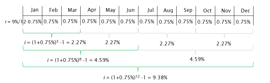
where i = the effective interest rate, or EIR, r = the nominal interest rate, or APR, C = the number of interest periods per payment period, and K = the number of payments per year. Given a nominal interest rate and compounding frequency, the EIR can be calculated for any payments schedule using formula 4.4. For example, for 9% APR, compounded monthly, the effective rates for monthly, quarterly, semi-annual, and annual payments are shown in Figure 4.2:
Figure 4.2 The Effective Interest Rate for Different Payment Frequencies Note that the EAR is a partial case of the more general form, the EIR. When payments are made annually, from equation 4.3 we get K=1 and, thus, M=C. Consequently, using the fact that M=C, we get the formula for EAR (4.2) from the formula for EIR (4.4). Similarly, the interest rate with compounding period is also a partial case of the EIR, when payment and compounding frequencies are the same. These partial cases together with the two cases when compounding frequency is higher than the payments frequency and when compounding frequency is lower than the payment frequency are explored in more detail in the example below. Effective Interest Rate Example: different compounding and payment frequencies scenarios Irvin has 4 savings accounts from different banks. The terms and payment schedules for these accounts are as follows:
What are the effective interest rates on each of these accounts? Solution This example represents 4 scenarios with the same nominal interest rate, but different compounding and payment frequencies. Account 1 In the first scenario, the interest is compounded monthly and payments are made monthly, so the compounding frequency is equal to the payment frequency. In this case, we use the interest rate per compounding period formula (4.1): we divide the nominal interest rate by the number of interest periods, which is equal to 12, to get the effective monthly interest rate for scenario 1:
Another way to get the EIR is to use the general EIR formula (4.4). We do this calculation to check the answer. Substituting r = 8%=0.08, C= 12 and K = 12, we get:
So, the effective monthly interest rate on the first savings account is 0.67%. Account 2 In the second scenario, the interest is compounded monthly and payments are made quarterly, so the compounding frequency is higher than the payment frequency. One payment period contains 3 interest periods. We use the general EIR formula (4.4) to calculate the effective interest rate per quarter. Substituting r = 8%=0.08, C= 3 and K = 4, we get
So, the effective interest rate per quarter on the second savings account is 2.01%. Account 3 In the third scenario, the interest is compounded quarterly and payments are made monthly, so the compounding frequency is lower than the payment frequency. One payment period contains of an interest period. Like in the previous scenario, we use the general EIR formula (4.4) to calculate the effective interest rate per month. Substituting r = 8%=0.08, C= and K = 12, we get:
So, the effective interest rate per month on the third savings account is 0.66%. Account 4 In the fourth scenario, interest is compounded monthly and payments are made annually, so payment are made once a year. Recall that this is a partial case when we calculate the effective annual rate (EAR) using formula 4.2 and M=C =12. The EAR is:
So, the effective annual rate on the fourth savings account is 8.30%. Summarized formulas for the 4 scenarios depending on compounding and payment frequency can be found in Table 4.3 below.
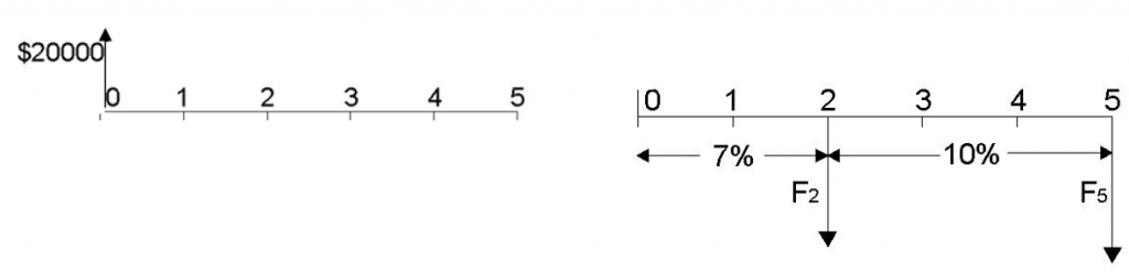
Table 4.3 Effective interest formulas for corresponding compounding-payment frequency scenarios Note that the Table 4.3 contains suggested formulas. In all four scenarios, the general EIR formula (4.4) can be used. The results will be the same. Which formula to use is just a matter of preference. 4.2.1.4 Changing Interest RatesPreviously in Sections 4.2.1.1 through 4.2.1.4 we assumed the same interest rate throughout the term of the loan. However, while the interest rate is fixed for many short-term loans, many long-term loans allow the interest rate to be adjusted. As discussed in Chapter 3, the interest rate is set to account for inflation and risks associated with borrowing money. In contrast to short-term loans, it is a lot harder to project inflation and risks over longer periods of time to guarantee a fixed interest rate. The economic situation in the region is subject to constant change: for example, when the inflation rate prognosis changes in 5 years due to government policy, the interest rates have to be adjusted accordingly. Thus, the ability to adjust interest rates is an important leverage to mitigate possible shocks and economic changes in the long run, and ensure the costs associated with borrowing money are met. How do we approach loan calculations when the interest rate changes throughout the term of the loan? Let’s take a look at an example that addresses this scenario. Example 4.3 Suppose a company decides to take a $20,000 loan for 5 years. The terms of the loan state 7% APR compounded monthly for the first 2 years and 10% APR compounded monthly for the last 3 years. Payments are made monthly. What is the total amount the company will have to pay in 5 years? Using the cash flow diagram, this problem can be represented in the following way:
Figure 4.3 The Cash Flow Diagram for Example 4.3 One way to approach problems that involve changing interest rates is to move the cash flows through each interest rate phase. We have two interest rate phases in this example: the 7% and 10% phases, which we will call Phase 1 and Phase 2 accordingly. Phase 1 The example provides an annual percentage rate, however compounding and payment frequency are not annual. Thus, we need to adjust the interest rate to account for different compounding and payment frequency by calculating the effective interest rate. To decide which formula to use for calculating the EIR, we look at the relationship between compounding and payment frequencies. In our scenario, the compounding frequency is equal to the payment frequency – monthly, so we calculate a partial EIR case – interest rate per compounding period, using formula 4.3:
The next step is t calculate the future value of the loan at year 2. Interest is compounded 12 times a year, so in 2 years it is compounded 24 times. Using the future-value formula 3.6 we get:
So, the future value of the loan at the end of phase 1 is $22,994.29 Phase 2 Using the same approach as in phase 1, we first calculate the interest rate per compounding period for phase 2:
Now we move the cash flow from year 2 to year 5 using the future-value formula 3.6. Notice that this time we use the future value of the loan at year 2 instead of present value of the loan. This is what we mean by moving the cash flow through each interest rate phase.
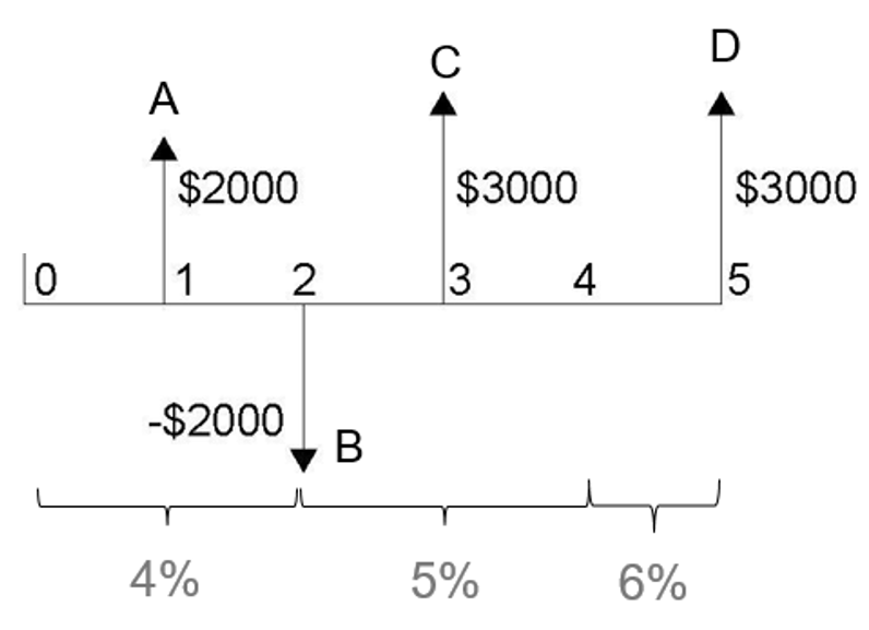
Thus, the total amount the company will have to pay in 5 years is $30,996.80. Changing Interest Rates Example What is the total present value of the payments shown in Figure 4.4? The following interest rates are all compounded annually.
Figure 4.4 Payments schedule Solution Step 1: To solve this problem, firstly, we have to move all payments individually through the interest periods. There are 4 payments A-D in the example. Because interest is compounded annually and payments are made annually, we do not have to adjust the interest rate. Payment A The first payment is made in year 1. We use the present-value formula 3.8 introduced in Chapter 3 to calculate the value of payment A in year 0:
Payment B In the second year, we have a negative cash flow. Movement of the payment to year 0 does not require changing interest rate, so we use the present-value formula 3.8 to obtain the present value of the cash flow:
Payment C To discount the value of the third payment in year 3, we now have to account for the changing interest rates. Thus, we first discount the payment using 5% interest rate to find the value of the payment in year 2, then discount the payment using 4% interest rate to find its value in year 0:
and You can also do this in one step:
Payment D Payment D is made in year 5. To discount this payment, we have to account for the interest rate changing 2 times: in year 4 and in year 3. Firstly, we discount the payment using 6% interest rate to find the value of the payment in year 4. Then we use 5% interest rate to move the payment to year 2. Finally, we use 4% interest rate to obtain a present value in year 0 of the payment. This could be done in multiple steps or in one step as follows. Multiple-step:
One step:
Step 2: Now that we know present values of all payments, we sum them to find the total present value of all payments:
So, the total present value of payments shown in Figure 4.4 is $5088.96.
|

![i=\left(1+\frac{r}{CK}\right)^C-1</td> <td style="width: 20.1px"> (4)</td> </tr> </tbody> </table> Thus, the formula for calculating the EAR is [latex]i=(1+\frac{r}{CK})^C-1](https://openpress.usask.ca/app/uploads/quicklatex/quicklatex.com-df00ba2ffe8318d8182c339a39e60733_l3.png "Rendered by QuickLaTeX.com") (4.4)
(4.4)