3.3 Economic Equivalence
We have just considered two key factors relating to the time value of money:
- Inflation, which explains the reduction in purchasing power over time; and
- Interest, which is the cost of borrowing money and helps maintain the lender’s purchasing power.
The TVM concept enables us to compare situations when financial transactions occur in different time periods. For example, would you prefer to get $500 now, $700 three years from now or $200 a year for the next three years? How would you decide? Are these three options equal?
When two sets of financial transactions yield the same outcome regardless of the timing of the transactions, the two are said to be economically equivalent. In other words, if there were two cash flows that occurred at different times and had the exact same effect on a person’s financial position, then the two cash flows would be economically equivalent. In these situations, we are indifferent to choosing one rather than the other.
Example 3.3
Let’s say that Adam can choose to receive $100 from Becky right now, or $105 a year from now, and he has access to a bank account that pays 5% interest compounded annually. He would be indifferent when choosing which amount to take: he could take the $105 a year from now, or he could take the $100 and deposit it into the bank account to earn $5 in interest and end up with a total of $105 in the bank after one year. Thus, the $100 cash flow and the $105 cash flow are economically equivalent.
3.3.1 Principles of Economic Equivalence
There are four key principles that always hold true and are fundamental to understanding economic equivalence and its application to financial decision-making.
Principle 1: Cash flow comparisons require a common time basis. Alternative cash flow scenarios must be compared within the same time period. This means we need to “move” cash flows to put them all in the same time period. Often, we compare the alternatives at the present time, but a future point in time may be used as well.
In example 3.3, we compared the two cash flows in the same time period as per principle 1. We applied interest to $100 in the current period to obtain the future value after one year using the future value formula introduced in the Interest section. This yields the future value of $105. As principle 1 states, we had to find the future value of the present cash flow for it to be comparable to the other cash flow that occurs one year from now. We then compared the two cash flows, arriving to conclusion that the two are economically equivalent.
Principle 2: Economic equivalence is dependent on the “discount rate”. To account for the time value of money while “moving” these cash flows we must reduce the economic value of future cash flows. Why? Recall that a dollar today is worth more than a dollar tomorrow, which means that a dollar tomorrow is worth less than a dollar today. So, when converting future cash flows to their equivalent (lower) present value to compare these cash flows we use what is termed a discount rate. (Note that the term discount rate is also used when converting cash flows to a future point in time.)
Note: A “discount rate” is the rate used to discount future cash flows to adjust for the time value of money. Generally, the discount rate is set to account for a cost (or group of costs) the investor or creditor may incur due to the investment. Depending on the context, the discount rate can be equivalent to the interest rate, for example when dealing with savings accounts or loans. Usually, however, the discount rate is higher than the interest rate, as it accounts for other costs as well, such as opportunity costs which will be covered in Chapter 5.
We will talk more about the discount rate and how it is set in chapter 5.
Changing the discount rate that is used to “move” cash flows to other time periods will change values of the respective cash flows. From example 3.3, if the interest rate was 10% instead of 5%, the future value of the $100 cash flow after one year would be $110. Comparing with the alternative $105 cash flow in the same time period, we see, that the two cash flows are no longer economically equivalent. Note, that we use the interest rate as the discount rate in this case to account for the time value of money.
Principle 3: Comparisons may require conversion to a single cash flow. When there are multiple cash flows to be considered in an alternative cash flow scenario, the individual cash flows may need to be combined into a singe cash flow for comparison. To illustrate this, let’s slightly modify example 3.3.
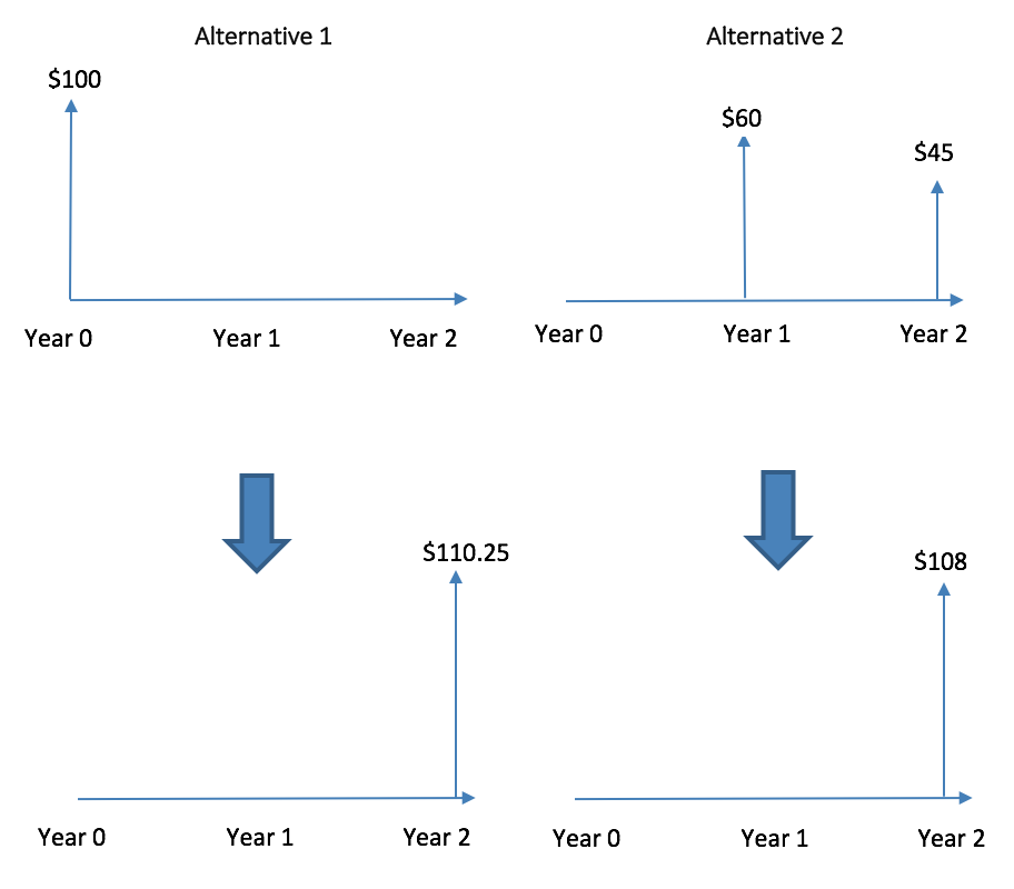
Say Adam now has to decide whether to receive $100 from Becky now or, as an alternative, $60 in the first year and $45 in the second year, as shown in the diagram below. Like before, he has access to a deposit account that pays 5% compounded annually.
This time, we must compare the single $100 cash flow to a multiple cash flow alternative. The future value of the $100 cash flow in 2 years is $110.25. As per principle 3, the future value of the alternative option is: $60*1.05+$45=$108. So, by converting the multiple cash flows to a single one we can see the two alternatives are not economically equivalent.
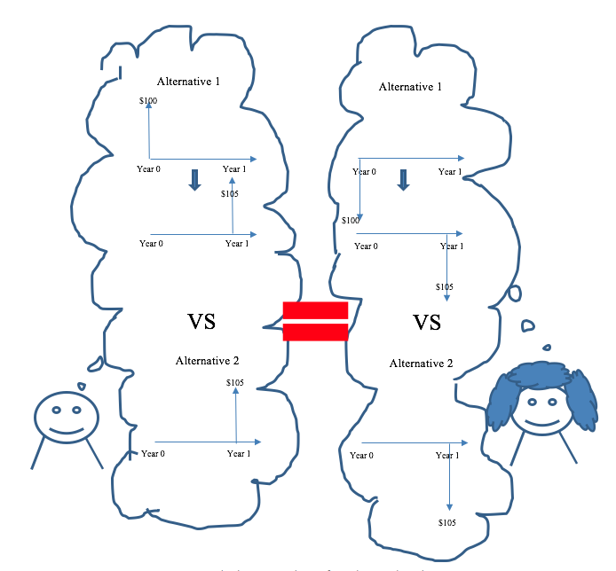
Principle 4: Equivalence is maintained regardless of point of view. As long as the same discount rate is used (see principle 2), the equivalence between cash flows will be maintained at any point in time to any party involved in the transactions. That is, it doesn’t matter if you are paying or receiving money. Economic equivalence will be the same from both perspectives.
Let’s analyze the cash flow diagrams from Adam’s and Becky’s point of view. From example 3.3 comparing $100 today and $105 a year from now with 5% interest compounded annually, as per principle four, the economic equivalence will be maintained for both Adam and Becky.