
6.1 Replacement Analysis
Any project or investment is bound to have a finite lifespan, after which it will require replacement. Often, the costs of a project will increase over time, which in many cases means the profitability decreases, and eventually the revenue or other benefits gained will be less than the expected profit of replacing it with a new investment. For example, it might be possible to keep your old refrigerator running for many years. However, the cost savings of replacing it with a newer, more energy-efficient model might eventually outpace the cost of buying that new fridge. Replacement analysis is used to determine when the cost of replacing a project is preferable to maintaining it.
The replacement does not need to be an identical project or investment. For instance, the original business model for Netflix was a DVD rental company which sent out movies to its customers by mail. As media trends changed, Netflix gradually replaced this model with a service to stream movies and television shows over the internet, and later began to produce their own original content. These decisions were based on an analysis of whether the replacements (the new services) would generate more long term revenue than the company’s existing investments.
Replacement analysis is closely related to the concept of opportunity costs discussed in Chapter 5: when your money is tied up in a project with a lower rate of return than another available project, you encounter the opportunity cost of not being able to pursue the more lucrative project. Replacement analysis allows you to determine when you should reinvest in a new project.
6.1.1 Economic Life vs. Physical Life
In Chapter 5, we introduced the linear depreciation method, which allowed us to estimate the salvage value of a project based on its original cost and the amount of time it had been in use. The assumption we made was that a project’s value is initially equal to its investment cost, and its value declines steadily over time. In this scenario, the amount of time before the project can no longer be used or its value reaches zero is referred to as its physical life. The physical life of a project is the amount of time it can operate while still generating economic value. For example, the physical life of a car is the number of years it can be run before breaking down irreparably.
As discussed in our introduction to replacement analysis, there are situations where we would rather replace a project before the end of its physical life. To build on previous example, the physical life of a car may be 25 years, but after 10 years of ownership we might choose to replace the car with a new vehicle that consumes less fuel and does not require expensive repairs (or just looks prettier). Let’s look purely at the economics: if after 10 years, these costs have finally surpassed the price of trading in the car for a new vehicle, then we say that the car has reached the end of its economic life. The economic life of an project is the period of time when it is generating greater value than any possible alternatives. A project’s economic life is always equal to or shorter than its physical life.
To generate the most economic value, we want to replace our projects at the end of their economic life, rather than at the end of their physical life. Identifying this optimum replacement point is the basic concept of replacement analysis.
Example #1
Sophie runs a printing company which produces books for large publishing houses. The facility she operates uses a set of old printing presses, and she expects that her business might become more profitable if she were to upgrade to newer, more reliable presses that would require less maintenance. Assume that her current set of presses are now valued at $400,000, and will depreciate linearly (to zero) until the end of their useful life in 25 years. In the next year, she predicts the presses will incur $40,000 in maintenance costs, and that this amount will increase by 10% each year as the presses age. She could upgrade right now to a new set of presses for $2,000,000; due to technological advances and more widespread use, over the next 10 years, the price of buying these new presses will decrease linearly to $1,000,000, and then remain at that price for the next 15 years. The new presses will require negligible maintenance, and the purchase price covers the long-term maintenance. The old set of presses earns $120,000 per year, and the new set would earn $300,000 per year. How long should Sophie wait before upgrading her presses? Use a MARR of 4%.
Step 1: The most useful way to visualize this problem is to create a table which finds the NPV of selling the presses each year. To do this, we consider 4 elements:
- the salvage value of the old presses,
- the expense of the new presses,
- the revenue from the old presses until they are sold, and
- the revenue from the new presses after they are bought.
We can find (1) by interpolating between $400,000 and $0 over 25 years for the old presses, and (2) by interpolating between $2,000,000 and $1,000,000 for the new presses over the same time period, as shown below in columns two and three. In the fourth column we use our basic present value formula to find the present value of the sum of the two previous columns. This should yield the following results:
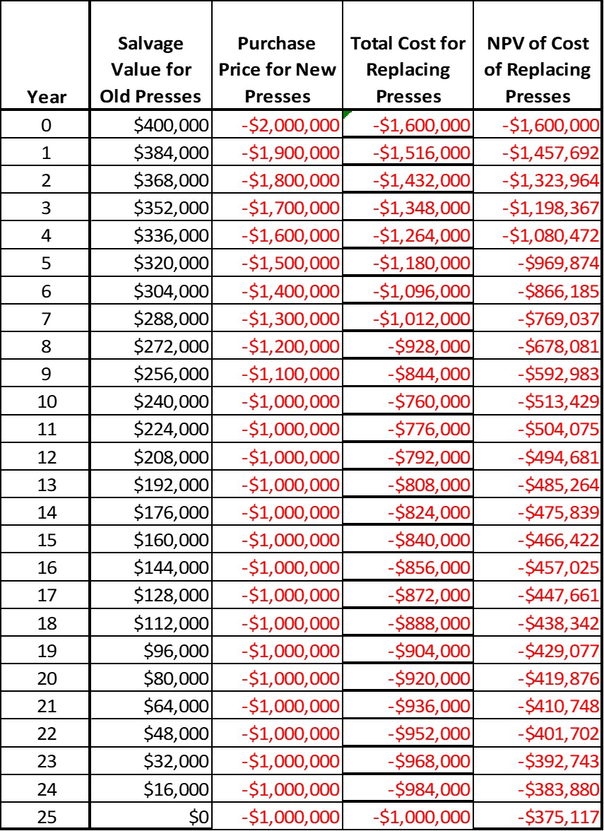
Table 6.1: Salvage values and expenses for replacing old printing presses
Step 2: Next, find the NPV of the elapsed maintenance costs each year using the geometric gradient series formula, and add this to the table:
![NPV_{Maintenance}=\frac{A}{i-g}\left[1-\left(\frac{1+g}{1+i}\right)^N\right]=\frac{\$1500}{0.04-0.1}\left[1-\left(\frac{1+0.1}{1+0.04}\right)^N\right]](https://openpress.usask.ca/app/uploads/quicklatex/quicklatex.com-c3a86e9e8fe56c8f095a3d62e3a0308f_l3.png "Rendered by QuickLaTeX.com")
Step 3: Next, find the NPV of the elapsed revenue from the old presses each year using the equation for a linear series:
![NPV_{OldRev}=A\left[\frac{(1+i)^N-1}{i(1+i)^N}\right]=\$120,000\left[\frac{(1+0.04)^N-1}{0.04(1+0.04)^N}\right]](https://openpress.usask.ca/app/uploads/quicklatex/quicklatex.com-e5a3594d13f0eec2172be5d0adc3ce29_l3.png "Rendered by QuickLaTeX.com")
Step 4: Finally, find the NPV of future revenue to be gained from the new presses in future years, by subtracting the value up to the current year from the value of a 25-year series:
![NPV_{NewRev}=\$300,000\left[\frac{(1+0.04)^{25}-1}{0.04(1+0.04)^{25}}\right]-\$300,000\left[\frac{(1+0.04)^N-1}{0.04(1+0.04)^N}\right]](https://openpress.usask.ca/app/uploads/quicklatex/quicklatex.com-d7bbeaa65907e9fca1a9670d28067caf_l3.png "Rendered by QuickLaTeX.com")
We can add all of these values to the table, and sum all of our NPVs to get a total NPV representing the value of switching to new presses during each year:
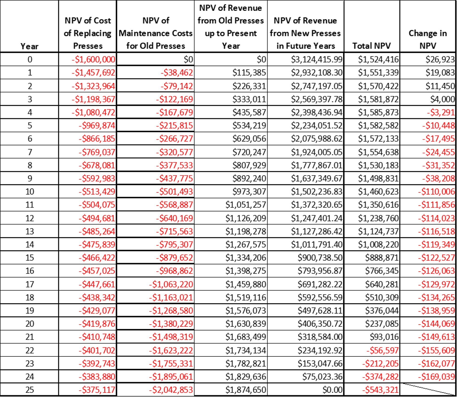
Table 6.2 Total net present value of the business each year, if the old printing presses were replaced in that year.
All of the NPV totals in the final column are positive, so we can conclude that switching to new presses would be lucrative move at any point in time. However, we can also see that the peak NPV value is at Year 6, with a maximum NPV of $1,544,345. If Sophie wants to create the maximum profit for her business, she should replace her printing presses at the end of their economic life in 6 years time.
Example #2
The youngest intern at the printing company, Paul, is convinced that printing books is a dying industry. Instead of investing in new printing presses, he believes the company should invest in a set of large-scale 3-D printers and shift its business model accordingly. This would be a much larger up-front investment than upgrading to new printing presses, because it would also involve replacing much of the other book-making equipment in the facility. He presents the projected costs and profits below to Sophie for her consideration. Sophie doesn’t want to spend too much time reviewing this proposal, so she only wants to check whether switching to 3-D printers now would be more profitable than keeping the old presses for the next 10 years (note that this is a different analysis period than was used in the previous question). Since Paul could not provide a reasonable estimate for 3-D printer salvage costs, she decides to ignore the salvage value of both alternatives. Using Sophie’s methodology, the estimates below, and the data from the previous question, evaluate Paul’s proposal.
| Paul’s 3-D Printer Estimates | |
| Equipment Purchase: | $3,250,000 |
| Annual Maintenance: | $5000/year |
| Annual Revenue: | $300,000 in year 1, increasing by 12% per year |
Table 6.3 Cost and revenue estimates for replacing the old printing presses with 3-D printers
Step 1: We can find the NPV after 10 years for the old presses by drawing from Table 6.1 we created in the previous question:
NPVOld = Maintenance NPV + Old Revenue NPV = -$18,806 + $973,307 = $954,501
Step 2: We can find the NPV of the 3-D printers by adding the purchase price to the NPV of the annual maintenance costs (a linear series) and annual revenue (a geometric gradient series):
![NPV_{3D}=P+A\left[\frac{(1+i)^N-1}{i(1+i)^N}\right]+\frac{A}{i-g}\left[1-\left(\frac{1+g}{1+i}\right)^N\right]](https://openpress.usask.ca/app/uploads/quicklatex/quicklatex.com-5aec2dc333c3fe3e93c81d5f9bb50b83_l3.png "Rendered by QuickLaTeX.com")

Since the NPV for the old presses ($954,501) is greater than for the 3-D printers ($827,695), Sophie would conclude that she should reject Paul’s suggestion and keep the old printing presses. However, since these results are very similar, and annual profits for 3-D printing appear to be rising more quickly than for book printing, Sophie should consider reviewing this analysis with better estimates and a more rigorous procedure.
