
5.4 Evaluation of Risk
In the examples we have covered so far, we have started out by saying things like “the project will have an annual revenue of $2000” or “the equipment will have a salvage value of $500 after 10 years”. But what if these assumptions are wrong? In reality, a project may not be worth what you initially expect, and this discrepancy introduces risk. Using a MARR for discounting cash flows allows us to roughly control for risk (as discussed in Section 5.1); but what about unforeseen circumstances that might create a large impact? For example, what if the economy slows down unexpectedly, reducing sales by 20% of a company’s estimate? What if the company’s borrowing rate changes? Consider the effect on businesses when the price of oil fell dramatically in 2014. Crude oil prices fell from $111 USD/barrel in June 2014 to $48 USD/barrel in January 2015, devastating Alberta’s provincial economy.
If the project you are undertaking has very certain outcomes, or will not have severe negative implications if unsuccessful, then you may be able to rely on the basic approaches we have covered already in this chapter. Otherwise, you will want to prepare for risk in your project. In this section, we will see how to analyze and account for risk.
Terminology
Here are some basic terms that will be used in this section.
- Risk: The chance that a project’s actual return will differ from its expected return.
- Risk analysis: Identifying and evaluating the impact of various risks on the financial success of a project.
- Base case: A scenario representing the most likely case for a project, where the value of all project variables and cash flows is set at an average estimate. We measure risk by comparing different scenarios to the base case.
- Break-even point: The value of a specific project variable at which the overall project transitions from unprofitable to profitable (i.e. the project’s NPV is 0)
- Scenario: A possible set of conditions for a project. Estimates of project variables can be adjusted to create and compare different scenarios.
Methods of Evaluating Risk
We will cover three methods for evaluating risk. Below, we list each method and its application. We will review each method in more detail in the following sections.
- Sensitivity analysis → Used for identifying the project variables that, when varied, have the largest effect on the value of the project.
- Scenario analysis → In this method, a project’s base case is compared to one or more alternative scenarios (such as the best and worst cases) to identify the most extreme and most likely possible outcomes.
- Break-even analysis → This method identifies the value of a particular project variable that would cause the project to break even.
5.4.1 Sensitivity Analysis
In sensitivity analysis, we want to find the variables that have the largest effect on the project’s value. For example, if you were opening a commercial bakery whose profits were very sensitive to the price of grain, and grain prices suddenly skyrocketed, your business could be in real trouble. So how do we apply this? Whichever value your decision is most sensitive to, you want to be as certain of as possible. You want to put extra time and effort into getting an accurate estimate. Starting with a reasonable range of values for the variables of your project is an extremely important step. If you are recommending a project to a manager, etc. you want to let them know your assumptions, what the decision relies on (e.g. this project is very sensitive to the price of oil).
There are two main types of sensitivity analysis: univariate analysis and multivariate analysis. In univariate analysis, we alter the value of only one variable at a time, while holding all others constant. In multivariate analysis, we alter the values of multiple variables at one time. In some cases, multivariate analysis can reflect more realistic risk scenarios (e.g. an increase in gasoline prices might cause cost variables for “shipping” and “sales overhead” to increase at the same time, if your salespeople are reimbursed for gas mileage). For the sake of simplicity, this chapter will only cover examples of univariate sensitivity analysis.
Here are the steps to performing univariate sensitivity analysis.
- Identify and list all variables that factor into the value of the project.
- Establish a base case of cash flow values and conditions that form a reasonable starting point for analysis. These are generally based on estimates of the most likely values.
- Analyze the project’s cash flows using the base-case values. This method of analysis may be NPV, AEV, etc.
- Set a range of possible values for each variable. This is the range of potential values in which the variable could fall. It is usually expressed as a percentage of the base value (e.g. a salvage value could be $15,000 ±20%) or a constant value (e.g. 10 years ±1 year).
- Adjust just one variable and recalculate the NPV of the project. Leave all other variables at their base-case values.
- Continue to adjust the same variable incrementally within its range, until the entire range is covered, recalculating the project’s NPV each time the variable is adjusted. When adjusting the variable, you will likely want to choose some intermediate points between the two extremes – for example, if the interest rate varies between 6% and 14%, you might calculate project NPVs setting the interest rate at 6%, 8%, 10%, 12%, and 14%. Note that in most cases you only need to test the extreme (highest and lowest) values of the range (e.g. 6% and 14%) because the relationship between the variable and the NPV is linear. If the relationship is non-linear, then you will need to calculate intermediate values.
- Repeat steps 5 and 6 for all other variables. Remember, when moving on to each new variable, to reset all other variables to their base-case values.
- Record each project NPV and its corresponding variable values. By examining the data, you can determine which variables have the greatest effect on the project’s NPV. We generally look at the extreme values for each variable; the variable which gives an NPV furthest from the base case NPV is the most sensitive.
- (Optional) Plot the data on a tornado or spider diagram to visually illustrate which variables have the greatest effect.
In the steps above, we defaulted to using NPV. However, note that sensitivity analysis can be used for more than just NPV – for example, it can also be used to calculate AEV. The general process for this is the same.
The key difference between univariate and multivariate analyses is that in Step 5 we may adjust the values of more than one variable at a time.
Displaying Sensitivity Analysis Results
As mentioned in the sensitivity analysis steps, there are two particularly useful charts for displaying the results of sensitivity analysis: sensitivity diagrams and tornado diagrams. Both can be done using a spreadsheet program. For example, the table of results shown in Figure 1 below could be used to generate the diagrams shown in Figures 2 and 3. You will notice that in this example, not all of the variables vary by the same amount. This is a realistic expectation, since some factors like fixed cost and demand might be more predictable than other variables under certain circumstances.
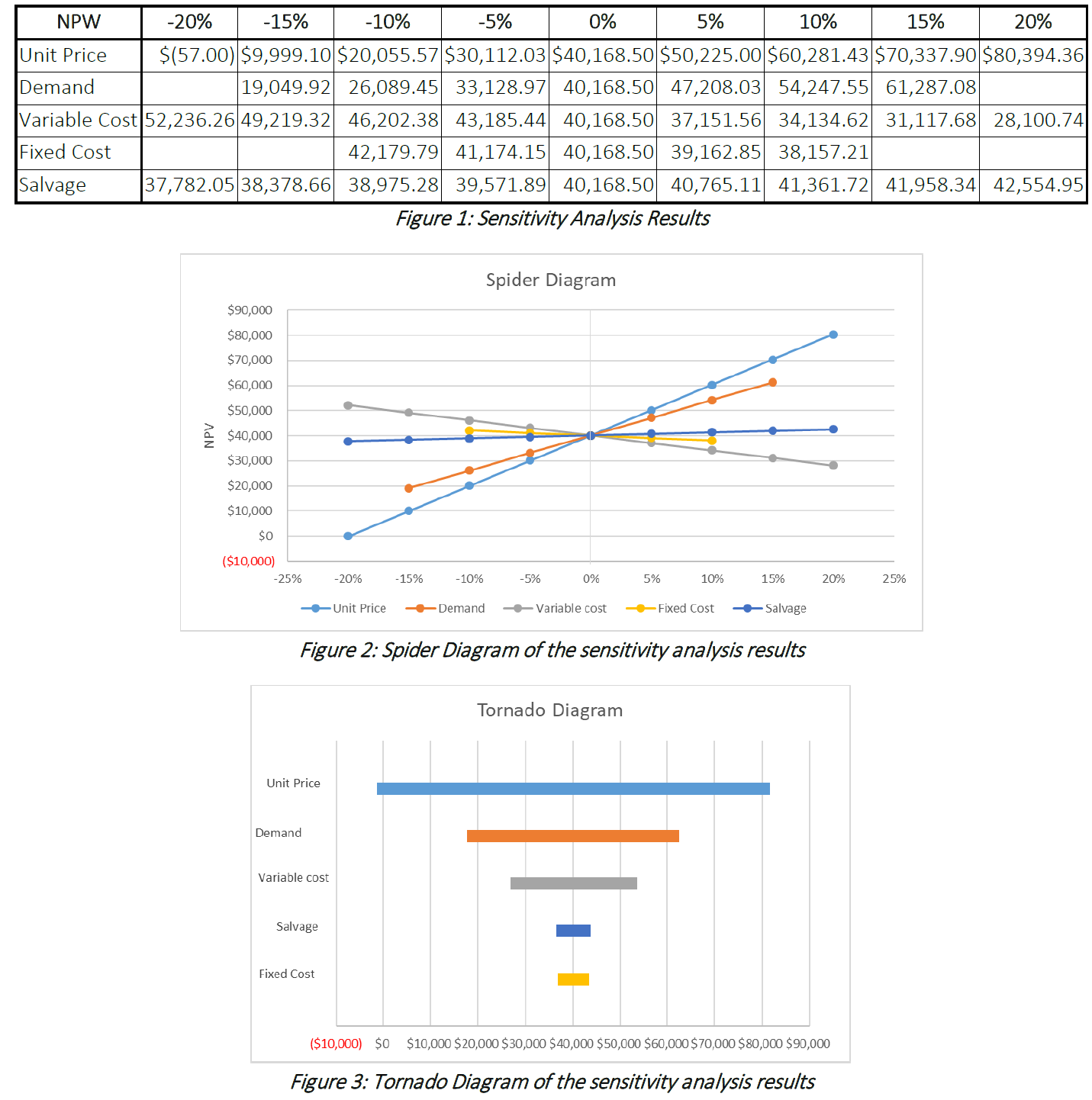
Sensitivity diagrams and tornado diagrams both illustrate the same concept: they show how the project’s NPV (or AEV, etc.) changes as the variables change. Each line shows how the project value changes as one variable is adjusted, keeping all other variables constant. The number of lines will be equal to the number of variables you are analyzing. The only thing that differs between the two diagrams is how they are presented.
In the sensitivity diagram, we plot project value on the y-axis, and the percent change of the variable along the x-axis. The point at which all lines intersect is the base-case value of the project. Once the data are plotted for each variable, we can see how each variable affects the project value (i.e. whether an increase in the variable causes an increase or decrease in project value, and by how much). The line with the steepest slope will generate the most extreme NPVs, and will reflect the variable which most significantly affects the value of the project. Similarly, a line with a mild slope will produce less extreme NPVs, and will reflect a less sensitive variable. Looking at the figure above, Unit Price is the most sensitive variable (steepest slope), and Salvage is the least sensitive variable.
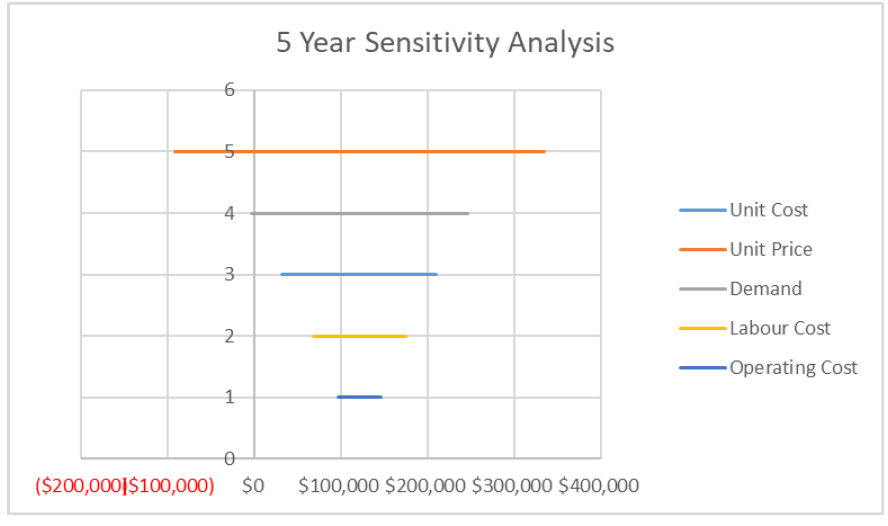
On a tornado diagram, the range of values for each variable is lines is plotted as a horizontal line, across the project values on the x-axis. On a tornado diagram, the longer a line is, the more the variable affects the project’s value. The lines are typically arranged by length, with the longest line at the top, so that the diagram resembles a tornado. As Figure ___ shows, Unit Price has the longest line, and is the most sensitive variable. The base-case NPV is noted by the vertical line on the diagram, which is in the exact centre of each horizontal line.
5.4.2 Scenario Analysis
Scenario analysis is an adapted form of sensitivity analysis. In scenario analysis, we compare scenarios – essentially sets of values for each variable in the project. The scenarios are based on the likely range of values for each variable, as well as the probability of each set of values. While it may be useful to check several combinations of variables, it should be noted that not all scenarios are feasible or likely, and so analyzing every possible scenario is unnecessary. For example, you would likely not consider a scenario where demand for your product is extremely low but your monthly shipping costs are extremely high, since your shipping costs should be somewhat dependent on the amount of product you are selling.
Scenario analysis allows you to prepare for the outcomes of multiple likely situations, and understand the most extreme impacts of the risks facing your project. It can also be a useful tool to help decision makers understand the risks and benefits of a project in a way that makes intuitive sense.
Here are the steps to performing a scenario analysis.
- Identify and list all variables that factor into the value of the project.
- Establish a base case scenario – a set of cash flow values and conditions that form a reasonable starting point for analysis. These are typically the most likely estimates for each variable.
- Calculate the NPV (or AEV, etc.) of the project for the base case scenario.
- Establish a new scenario. For each scenario being analyzed, obtain (or estimate) the values of all variables. Most often, we use a best-case and a worst-case scenario.
- Use the scenario from Step 4 to calculate the NPV of the project.
- Repeat steps 4 and 5 for all relevant scenarios.
- Compare the NPV of all scenarios, including the base case scenario.
As with sensitivity analysis, it is not necessary to use NPV as the measure of a project; AEV or another analysis method can also be substituted.
The goal of scenario analysis is to identify the most extreme (best and worst case) and most likely project outcomes. It might not be sufficient to only consider the best and worst case, especially if the best and worst case are both highly unlikely. It may be most useful to add more (and, hopefully, highly probable) scenarios by considering other known conditions surrounding the project.
5.4.3 Break-Even Analysis
Sometimes we are interested in how much our costs would have to increase, or how much our revenues would have to decrease, before a project begins to lose money. In these cases, we can use break-even analysis. Break-even analysis tells us what value of a particular variable will cause the project to exactly break even. Imagine that you run a bicycle repair shop, and you discover that your business will only break even if you charge at least $60 per repair. Or that at your current prices, you could increase your employees’ wages to $21/hour before your business began to lose money. These pieces of information could be very valuable to you when making decisions about pricing and employee salaries.
Break-even analysis is another valuable tool for informing decisions about businesses and projects, especially when considering a new project to invest in. Understanding the changes to certain variables that will make a project profitable gives a good basic indication of whether it is worth investment.
Here are the steps to performing break-even analysis:
- Identify and list all variables that factor into the value of the project.
- Establish a base case – a set of cash flow values and conditions that form a reasonable starting point for analysis.
- Determine a formula for the project’s NPV.
- Set the NPV equal to zero, and solve for a chosen “test” variable.
- Calculate the value of the test variable*. This will be the break-even point for the test variable. Make sure all other variables are held at their base-case values, and the NPV is zero.
- Repeat steps 4 and 5 for each variable. Each time you choose a new variable, remember to reset all other variables’ values to their base-case values.
*Note about step 5: Usually, the variable can be solved for directly. However, if the variable in question appears in multiple places in the equation, and can’t be isolated (this is common for the discount rate), special methods will have to be used. If this is the case, you may have to perform iteration. Excel is particularly helpful in this regard. You may have to look up fixed-point iteration or another, more advanced method to iterate in Excel.
Break-even analysis allows us to see how much we can allow each variable to change before we will refuse the project. If the break-even point falls within the estimated range of any of the variables, the project should probably be rejected. For example, if we expect unit costs to be somewhere between $18 and $22, and the project breaks even with unit costs of $21, the project may be too risky to undertake.
5.5.1 Example of Sensitivity, Scenario and Break-Even Analysis
Sensitivity Analysis: 1-year
To begin the sensitivity analysis, create a table of cash flows for the project, calculating the NPV of the project over its duration. Begin by using the base case values supplied for all variables. Your table could look something like this:
| Year | 0 | 1 |
| Revenues: | ||
| Unit Price | $6.00 | |
| Demand | 35,000 | |
| Sales Revenue | $210,000.00 | |
| Salvage Value | $150,000.00 | |
| Expenses: | ||
| Investment | $200,000.00 | |
| Unit Cost | $2.50 | |
| Demand | 35,000 | |
| Sales Cost | $87,500.00 | |
| Labour Cost | $60,000.00 | |
| Operating Cost | $30,000.00 | |
| Net Profit | -$200,000.00 | $182,503.50 |
| Net Present Value | -$200,000.00 | $175,484.13 |
| Total NPV: | -$24,515.87 |
The total NPW you calculate with this table represents a single data point for this analysis. To fill in the additional data points, you must alter the value of a single variable (e.g. Unit Cost) at a time, and find how a certain change (e.g. +5%) impacts the total NPV. For the purposes of this example, we will evaluate all of our variables in the range of ±20%, with increments of 5%. After evaluating every scenario for every variable, you should arrive at a table of results like this:
| -20% | -15% | -10% | -5% | 0% | 5% | 10% | 15% | 20% | |
| Unit Cost | -$7,688.46 | -$11,895.31 | -$16,102.16 | -$20,309.01 | -$24,515.87 | -$28,722.72 | -$32,929.57 | -$37,136.42 | -$41,343.27 |
| Unit Price | -$64,901.63 | -$54,805.19 | -$44,708.75 | -$34,612.31 | -$24,515.87 | -$14,419.42 | -$4,322.98 | $5,773.46 | $15,869.90 |
| Demand | -$48,073.56 | -$42,184.13 | -$36,294.71 | -$30,405.29 | -$24,515.87 | -$18,626.44 | -$12,737.02 | -$6,847.60 | -$958.17 |
| Labour Cost | -$12,977.40 | -$15,862.02 | -$18,746.63 | -$21,631.25 | -$24,515.87 | -$27,400.48 | -$30,285.10 | -$33,169.71 | -$36,054.33 |
| Operating Cost | -$18,746.63 | -$20,188.94 | -$21,631.25 | -$23,073.56 | -$24,515.87 | -$25,958.17 | -$27,400.48 | -$28,842.79 | -$30,285.10 |
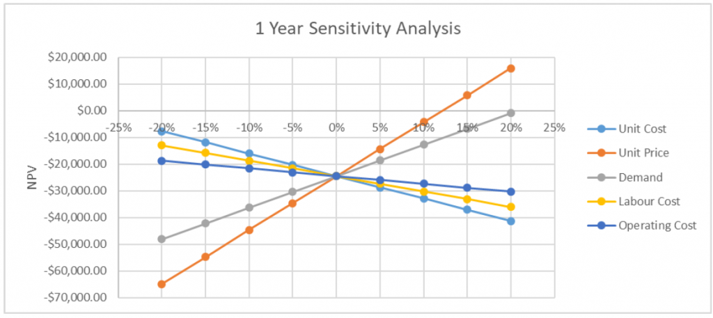
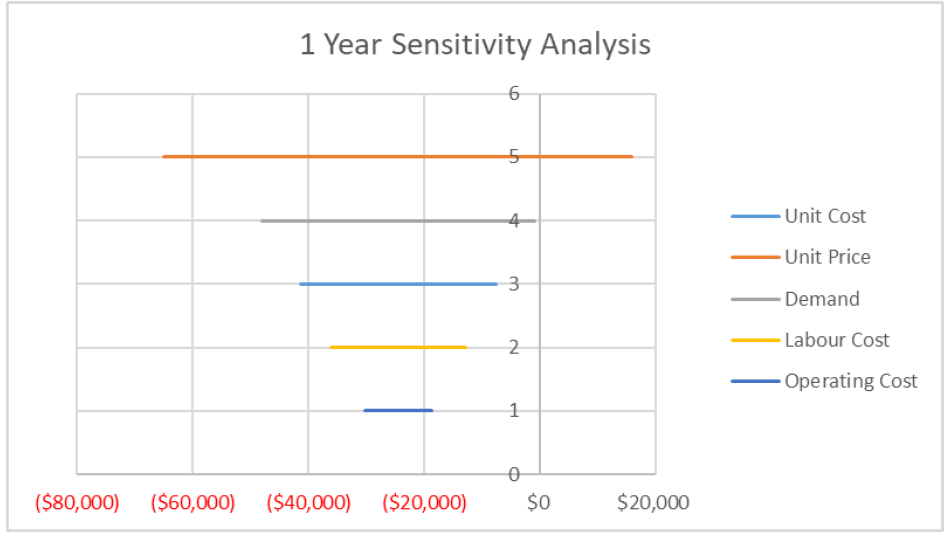
We can display the results of a sensitivity analysis graphically using either a sensitivity diagram or a tornado plot. This can be accomplished in a spreadsheet program by isolating the important results from each variable as inputs for a graph:
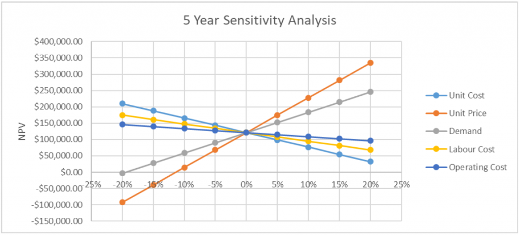
Sensitivity Analysis: 5 year
If we follow the same methodology for our 5-year estimates, we should produce the following results and graphs.
| Year | 0 | 1 | 2 | 3 | 4 | 5 |
| Revenues: | ||||||
| Unit Price | $6.00 | $6.00 | $6.00 | $6.00 | $6.00 | |
| Demand | 40,000 | 40,000 | 40,000 | 40,000 | 40,000 | |
| Sales Revenue | $240,000.00 | $240,000.00 | $240,000.00 | $240,000.00 | $240,000.00 | |
| Salvage Value | $120,000 | |||||
| Expenses: | ||||||
| Investment | $200,000.00 | |||||
| Unit Cost | $2.50 | $2.50 | $2.50 | $2.50 | $2.50 | |
| Demand | 40,000 | 40,000 | 40,000 | 40,000 | 40,000 | |
| Sales Cost | $100,000.00 | $100,000.00 | $100,000.00 | $100,000.00 | $100,000.00 | |
| Labour Cost | $60,000.00 | $60,000.00 | $60,000.00 | $60,000.00 | $60,000.00 | |
| Operating Cost | $30,000.00 | $30,000.00 | $30,000.00 | $30,000.00 | $30,000.00 | |
| Net Profit | -$200,000.00 | $50,003.50 | $50,003.50 | $50,003.50 | $50,003.50 | $170,003.50 |
| Net Present Value | -$200,000.00 | $48,080.29 | $46,231.05 | $44,452.93 | $42,743.20 | $139,730.48 |
| Total NPV: | $121,237.95 |
| -20% | -15% | -10% | -5% | 0% | 5% | 10% | 15% | 20% | |
| Unit Cost | $210,276.62 | $188,016.96 | $165,757.29 | $143,497.62 | $121,237.95 | $98,978.28 | $76,718.61 | $54,458.95 | $32,199.28 |
| Unit Price | -$92,454.86 | -$39,031.66 | $14,391.54 | $67,814.75 | $121,237.95 | $174,661.15 | $228,084.36 | $281,507.56 | $334,930.76 |
| Demand | -$3,413.07 | $27,749.68 | $58,912.44 | $90,075.19 | $121,237.95 | $152,400.71 | $183,563.46 | $214,726.22 | $245,888.98 |
| Labour Cost | $174,659.82 | $161,304.35 | $147,948.88 | $134,593.42 | $121,237.95 | $107,882.48 | $94,527.02 | $81,171.55 | $67,816.08 |
| Operating Cost | $146,018.07 | $139,823.04 | $133,628.01 | $127,432.98 | $121,237.95 | $115,042.92 | $108,847.89 | $102,652.86 | $96,457.83 |
Scenario Analysis
To conduct a scenario analysis, we return to the same table of cash flows we used to compute our sensitivity analysis, and reference the either all of the provided best case values, or all of the provided worst case values, in order calculate a total NPV for the project. We will also include the base case calculation (completed during sensitivity analysis) for reference. This process should produce the following set of NPV values:
| 1-Year | 5-Year | |
| Best Case: | $126,928.85 | $794,589.43 |
| Worst Case: | -$137,499.04 | -$552,113.53 |
| Base Case: | -$24,515.87 | $121,237.95 |
Break-Even Analysis
To begin break-even analysis, we return our entire table of cash flows to its base case values. Then, for a single variable (e.g. Unit Cost), we determine what value it would need to hold for the total NPV of the project to equal zero (i.e. the break-even point), with all other base case values remaining constant. We could accomplish this by writing out a long equation for the NPV, setting it equal to zero, and then solving for our isolated variable. However, this process would be very time intensive, and if you are using a spreadsheet computer program, there will analysis methods you can run to quickly solve for the value of each variable.
This process should produce the following set of breakeven points:
| Break-even Point | 1-Year | 5-Year |
| Unit Cost | $1.77 | $3.18 |
| Unit Proce | $6.73 | $5.32 |
| Demand | 42,285 | 32,219 |
| Labour Cost | $34,503.50 | $87,233.33 |
| Operating Cost | $4,503.50 | $57,233.33 |
Conclusions
From the sensitivity analysis, we can conclude that unit price and demand are the two most sensitive variables, and also the only two variables that over 5-years have the potential to generate a negative NPV for the project. From this, we can conclude that setting a high enough price for the hamburgers is very important to the profitability of the business. However, we should also consider the real-world relationship between the price of the burgers and the demand for them; finding a suitably high price that will not hinder demand for your product will be one of the most important considerations for this business.
We can also see that the majority of values generated in this analysis, including the base case, for the 1-year estimates are negative, while for the 5-year estimates the majority are positive. This is largely due to the salvage value of the food trucks falling by $50,000 in the first year, and thus making it difficult to generate a net profit on the business with only one year of sales. We can conclude that this business is a safer and more lucrative investment over 5-years, and likely not even worth investment on a 1-year basis.
From the scenario analysis, we can conclude that there is a wide range of possible outcomes for this business, ranging from extremely profitable (almost quadrupling the initial investment in 5 years) to extremely unprofitable (losing on net around $500,000). While our sensitivity analysis showed us that this is likely to be a fairly safe investment, the potential for multiple negative variables to add up means that this project could lose a significant amount of money in a worst-case scenario. A 1-year investment involves less catastrophic risk, but because its base case still gives a negative NPV it would not be a wise investment. If you were investing your own savings in this business, you might consider the potential risk for a 5-year term to be too high to consider investing.
Finally, the break-even analysis provides us with useful values for the operation of the business. For example, if after opening the business, the unit cost of your burgers were to rise above its break-even point, you would know that you were at risk of having a negative project NPV. You could then adjust your business practices to correct for this, by increasing burger prices, running advertising to increase sales, reducing operating hours to limit labour costs, or seeking ways to operate the food truck equipment on a lower budget.
If we were attempting to make the business profitable on a 1-year basis, we can see that adjusting some variables would be more realistic than attempting to adjust others. Finding cheaper ingredients to reduce hamburger costs to $1.77/unit, or raising prices to $6.73/burger seems reasonable, but reducing operating costs to below $4,503 (an 85% reduction) would be nearly impossible.
